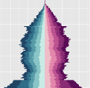

The IBMPopSim package aims at simulating the random evolution of heterogeneous populations, called stochastic Individual Based Models (IBMs). Such models have a wide range of applications in various fields including actuarial sciences, biology, demography, or ecology. For instance, IBMs can be used for simulating the evolution of an heterogeneous insurance portfolio, of an spatial ecological population with interacting individuals, or for validation mortality forecasts.
The package allows users to simulate population evolution in which individuals are characterized by their age and some characteristics, and where the population is modified by different types of events including births/arrivals, death/exit events, or changes of characteristics. The frequency at which an event can occur to an individual can depend on his age and characteristics, but also on time and on the rest of the population (interactions).
IBMPopSim overcomes the limitations of time consuming IBMs
simulations. This is done by implementing new efficient algorithms based
on thinning methods, which are compiled using the Rcpp library. The package allows a wide
range of IMBs to be simulated, while being user-friendly thanks to its
structure based on simple build blocks. In addition, we provide tools
for analyzing outputs, such a age-pyramids or life tables obtained from
the simulated data, consistent with the data format of packages for
mortality modeling such as StMoMo. See
vignette(IBMPopSim) for more details.
The latest stable version can be installed from CRAN:
install.packages('IBMPopSim')The latest development version can be installed from github:
# install.packages("devtools")
devtools::install_github('DaphneGiorgi/IBMPopSim')To illustrate the use of the package and to check the installation, a simple model with Poisson arrivals and exits is implemented.
library(IBMPopSim)

init_size <- 100000
pop <- population(data.frame(birth = rep(0, init_size), death = NA))

birth = mk_event_poisson(type = 'birth', intensity = 'lambda')
death = mk_event_poisson(type = 'death', intensity = 'mu')
params = list('lambda' = 100, 'mu' = 100)

# mk_model compiles C++ code using sourceCpp from Rcpp
birth_death <- mk_model(events = list(birth, death),
                        parameters = params)
If there are no errors then the C++ built environment is compatible
with the package. The model is created and a C++ code has been compiled.
The simulation is done using the popsim function.
sim_out <- popsim(model = birth_death,
                  initial_population = pop,
                  events_bounds = c('birth' = params$lambda, 'death' = params$mu),
                  parameters = params,
                  time = 10)

num_births <- length(sim_out$population$birth) - init_size
num_deaths <- sum(!is.na(sim_out$population$death))
print(c("births" = num_births, "deaths" = num_deaths))
## births deaths
## 952 981pop <- population(EW_pop_14$sample)params <- list("alpha" = 0.008, "beta" = 0.02, "p_male" = 0.51,
"birth_rate" = stepfun(c(15,40), c(0,0.05,0)))death_event <- mk_event_individual(type = "death",
intensity_code = "result = alpha * exp(beta * age(I, t));")
birth_event <- mk_event_individual(type = "birth",
intensity_code = "result = birth_rate(age(I,t));",
kernel_code = "newI.male = CUnif(0, 1) < p_male;")Note that these events contain some C++ statements that depend
(implicitly) on the previously declared parameters in variable
params.
mk_model. A C++ source code is obtained from the events and
parameters, then compiled using the sourceCpp function of
the Rcpp package. model <- mk_model(characteristics = get_characteristics(pop),
events = list(death_event, birth_event),
parameters = params)T bounds on the events intensities have to be
specified:a_max <- 115
events_bounds = c("death" = params$alpha * exp(params$beta * a_max),
"birth" = max(params$birth_rate))Then, the function popsim can be called:
sim_out <- popsim(model, pop, events_bounds, params,
age_max = a_max, time = 30)sim_out$population contains the
information (date of birth, date of death, gender) on individuals who
lived in the population over the period [0, 30]. Functions of the
package allows to provide aggregated information on the population.pop_out <- sim_out$population
head(pop_out)
## birth death male
## 1 -84.96043 NA FALSE
## 2 -84.86327 NA FALSE
## 3 -84.84161 NA FALSE
## 4 -84.79779 NA FALSE
## 5 -84.76461 NA FALSE
## 6 -84.76363 NA FALSE
female_pop <- pop_out[pop_out$male==FALSE, ]
age_pyramid(female_pop, ages = 85:90, time = 30)
## age male value
## 1 85 - 86 FALSE 224
## 2 86 - 87 FALSE 250
## 3 87 - 88 FALSE 213
## 4 88 - 89 FALSE 170
## 5 89 - 90 FALSE 180
Dxt <- death_table(female_pop, ages = 85:90, period = 20:30)
Ext <- exposure_table(female_pop, ages = 85:90, period = 20:30)params$beta <- 0.01
# Update death event bound:
events_bounds["death"] <- params$alpha * exp(params$beta * a_max)
sim_out <- popsim(model, pop, events_bounds, params,
age_max = a_max, time = 30)