
![]()
![]()
Bayesian learning is built on an assumption that the model space contains a true reflection of the data generating mechanism. This assumption can be problematic in complex data environments. By using a Bayesian non-parametric approach to learning, we no longer have to assume that the model is true.
This package implements a non-parametric statistical model using a parallelised Monte Carlo sampling scheme. The method implemented in this package allows non-parametric inference to be regularized for small sample sizes, while also being more accurate than approximations such as variational Bayes.
The concentration parameter is an effective sample size parameter, determining the faith we have in the model versus the data. When the concentration is low, the samples are close to the exact Bayesian logistic regression method; when the concentration is high, the samples are close to the simplified variational Bayes logistic regression.
This package is available on CRAN. The latest release can be installed using
install.packages("PosteriorBootstrap")If you prefer to use the bleeding edge version, you can install from
Github with devtools:
requireNamespace("devtools", quietly = TRUE)
devtools::install_github("https://github.com/alan-turing-institute/PosteriorBootstrap/")Please see the provided vignette (at vignettes/PosteriorBootstrap.Rmd)
for an example usage of the package to fit a logistic regression model
to the Statlog German Credit dataset.
The vignette reproduces Figure 2, page 8, from Lyddon, Walker, and
Holmes (2018), “Nonparametric learning from Bayesian models with
randomized objective functions” (32nd Conference on Neural Information
Processing Systems, Montréal, Canada). The vignette is limited to a
concentration parameter of c = 500 and the figure below
reproduces the one from the paper with the same concentration
parameters.
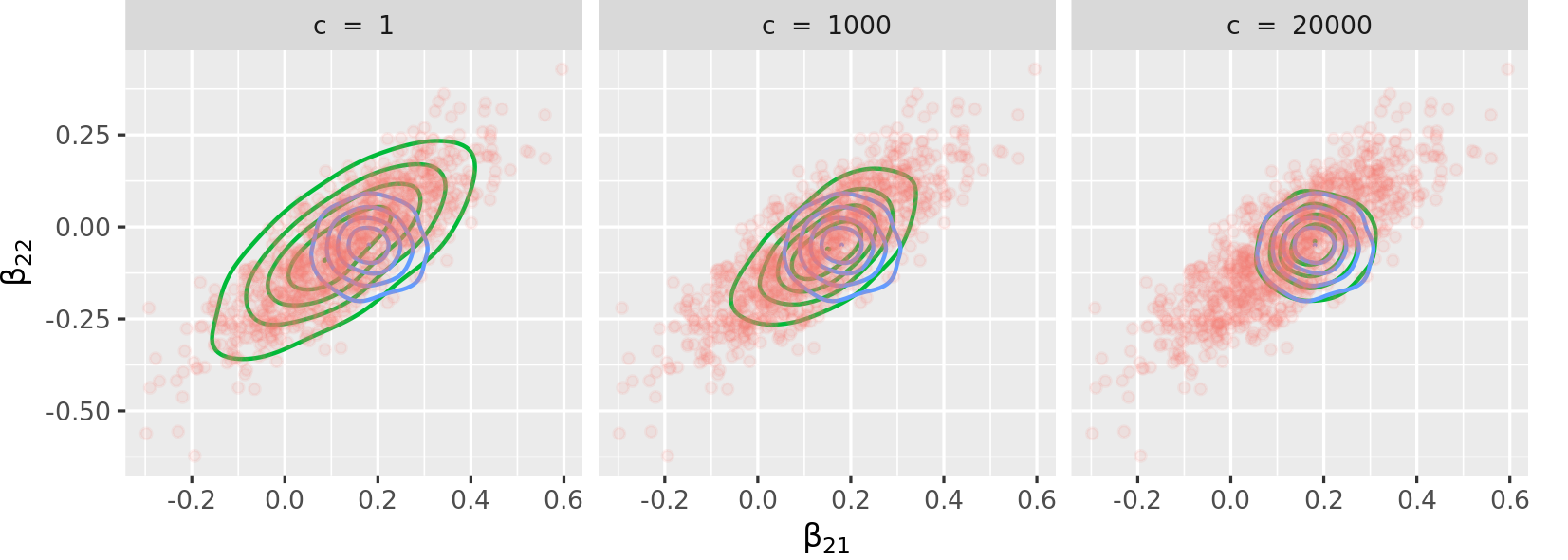
The figure above shows the advantage of the package: one can tune the
proximity of the sampling method to exact inference (Bayesian logistic
regression) with a low c or to approximate inference
(variational inference) with high c, or anywhere in
between. As mentioned in page 3 of the paper, the concentration
parameter c is an effective sample size, governing the
trust we have in the parametric model.
For any bug reports or feature requests, please open an issue on Github.
The calculation of the expected speedup depends on the number of bootstrap samples and the number of processors. It also depends on the system: it is larger on macOS than on Linux, with some variation depending on the version of R. Please note that parallelisation is currently unsupported on Windows.
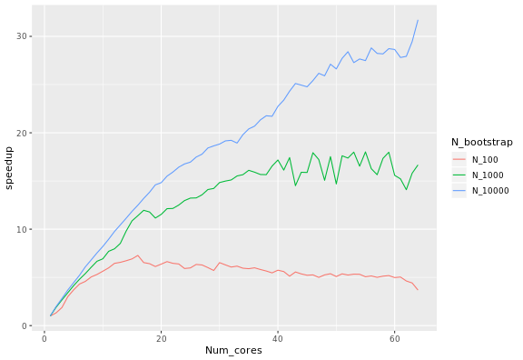
Fixing the number of samples corresponds to Ahmdal’s law,
or the speedup in the task as a function of the number of processors.
The speedup S_latency of N processors is
defined as the duration of the task with one core divided by the
duration of the task with N processors. When using 100,
1000 and 10000 samples, the following speed-ups were observed:
Inverting Ahmdal’s law gives the proportion of the execution time that is parallelisable from the speedup:
where S_latency is the execution speedup for the whole
task (as defined above), and s is the speedup for the part
of the task that can be parallelised. In this case, s is
simply equal to the number of cores used, so repeatedly measuring
S_latency for several choices of number of cores gives this
plot:
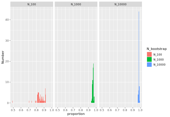
The proportion of the code that can be parallelised is high, and
higher the large the bootstrap samples, and always below 1. For large
samples with n_bootstrap = 10000, the values are close to
100%.
To run the results in this section automatically, you’ll need a Microsoft Azure subscription (one of the free subscriptions for example) and the Azure Command-Line Interface (CLI). You will need to login to your Azure account with the Azure CLI:
az loginthen follow the instructions. You will need to create a resource
group on portal.azure.com and
make note of the name of the resource group. The default name of the
resource group is PB for PosteriorBootstrap.
Then run the following on a shell with current directory at the root of the repository for deploying on a new machine:
azure/deploy.sh -g=<name of resource group> -k=<path to your private key>or, to deploy on an existing machine:
azure/deploy.sh -i=<IP address> -g=<name of resource group> -k=<path to your private key>The path to your private key defaults to ~/.ssh/azure if
you do not specify it, and the public key is that path with the suffix
.pub.
If you need to generate a private-public key pair, run:
ssh-keygen -t rsa -b 4096 -f ~/.ssh/azure