Penalized Regression with Second-Generation P-Values
We know that p-values can’t be used for variable selection. However, you can do so with second-generation p-values. Here is how.
To install it on CRAN, you can do
install.packages("ProSGPV")For a development version of ProSGPV, you can install it by running the following command.
library(devtools)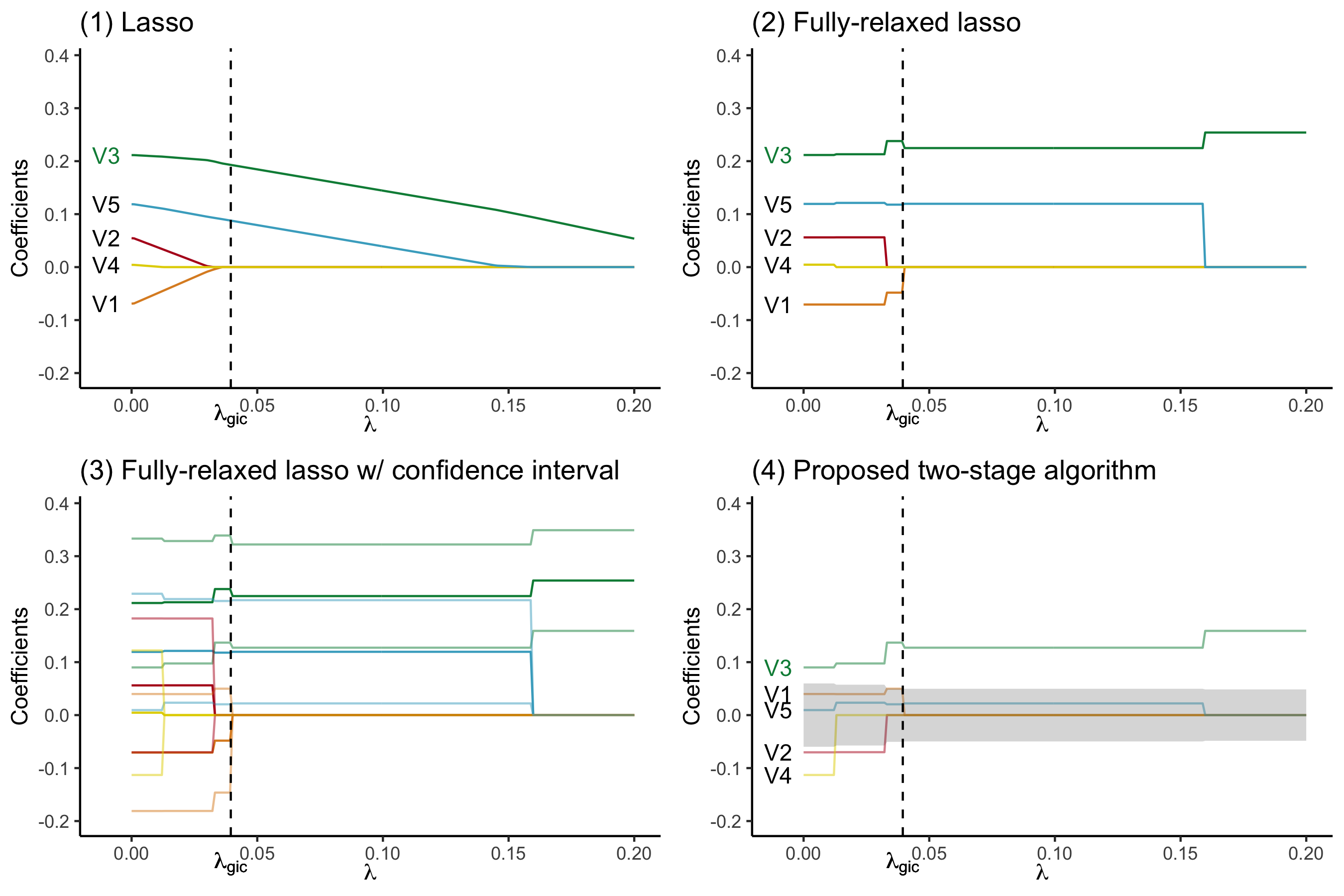
devtools::install_github("zuoyi93/ProSGPV")Below is an illustration of how ProSGPV successfully selects the true support, while lasso and fully relaxed lasso fails. Five variables are simulated and only V3 is associated with the response. Plot (1) presents the lasso solution path. The vertical dotted line is the lambda selected by generalized information criterion. (2) shows the fully relaxed lasso path. (3) shows the fully relaxed lasso paths with their 95% confidence intervals (in lighter color). (4) illustrates the ProSGPV algorithm selection path. The shaded area is the null region; the colored lines are each 95% confidence bound that is closer to the null region. Lasso and fully relaxed lasso would select both V5 and V3, while ProSGPV successfully screens out V2.
Here, we use the Tehran housing data as an illustrative real-world data example of how ProSGPV works with linear regression.
The Tehran housing data contain 26 explanatory variables and one outcome. Details about data collection can be found in this paper, and variable description can be found here.
We can load the Tehran Housing data t.housing stored in
the package.
# load the package
library(ProSGPV)

# prepare the data
x = t.housing[,-ncol(t.housing)]
y = t.housing$V9

# run ProSGPV
out.sgpv.2 <- pro.sgpv(x = x, y = y)
The two-stage algorithm selects the following variables.
out.sgpv.2#> Selected variables are V8 V12 V13 V15 V17 V26We can view the summary of the final model.
summary(out.sgpv.2)#>
#> Call:
#> lm(formula = Response ~ ., data = data.d)
#>
#> Residuals:
#> Min 1Q Median 3Q Max
#> -1276.35 -75.59 -9.58 59.46 1426.22
#>
#> Coefficients:
#> Estimate Std. Error t value Pr(>|t|)
#> (Intercept) 1.708e+02 3.471e+01 4.920 1.31e-06 ***
#> V8 1.211e+00 1.326e-02 91.277 < 2e-16 ***
#> V12 -2.737e+01 2.470e+00 -11.079 < 2e-16 ***
#> V13 2.185e+01 2.105e+00 10.381 < 2e-16 ***
#> V15 2.041e-03 1.484e-04 13.756 < 2e-16 ***
#> V17 -3.459e+00 8.795e-01 -3.934 0.00010 ***
#> V26 -4.683e+00 1.780e+00 -2.630 0.00889 **
#> ---
#> Signif. codes: 0 '***' 0.001 '**' 0.01 '*' 0.05 '.' 0.1 ' ' 1
#>
#> Residual standard error: 194.8 on 365 degrees of freedom
#> Multiple R-squared: 0.9743, Adjusted R-squared: 0.9739
#> F-statistic: 2310 on 6 and 365 DF, p-value: < 2.2e-16Coefficient estimates can be extracted by use of
coef.
coef(out.sgpv.2s)#> [1] 0.000000000 0.000000000 0.000000000 0.000000000 0.000000000
#> [6] 0.000000000 1.210755031 0.000000000 -27.367601037 21.853920174
#> [11] 0.000000000 0.002040784 0.000000000 -3.459496972 0.000000000
#> [16] 0.000000000 0.000000000 0.000000000 0.000000000 0.000000000
#> [21] 0.000000000 0.000000000 -4.683172725 0.000000000 0.000000000
#> [26] 0.000000000In-sample prediction can be made using S3 method predict
and an external sample can be provided to make out-of-sample prediction
with an argument of newx in the predict function.
head(predict(out.sgpv.2s))#> 1 2 3 4 5 6
#> 1565.7505 3573.7793 741.7576 212.1297 5966.1682 5724.0172S3 method plot can be used to visualize the variable
selection process.
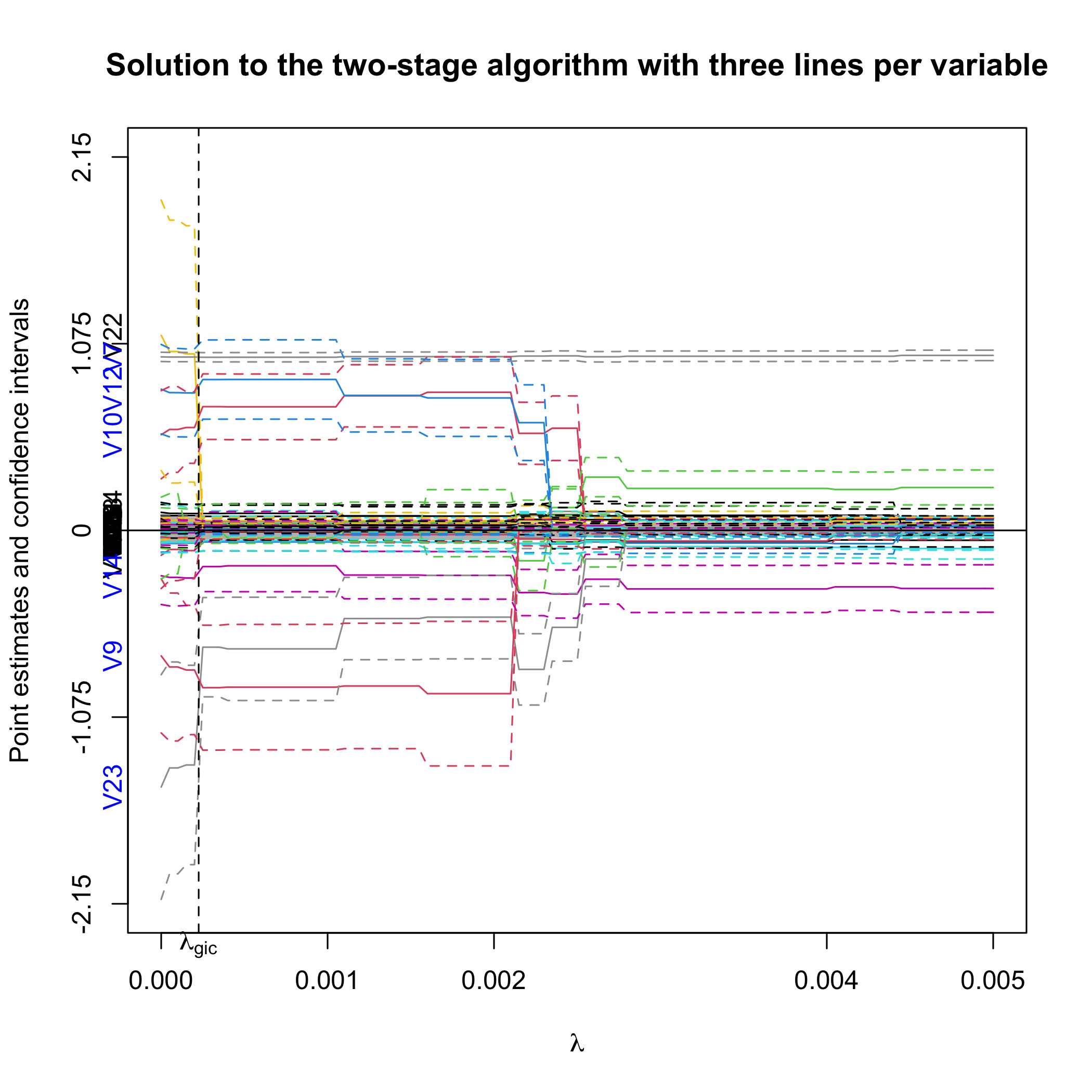
plot(out.sgpv.2, lambda.max = 0.01)First, we plot the full solution path with point estimates and 95%
confidence intervals. Note that the null region is in grey. The selected
variables are colored blue on the y-axis. lambda.max
controls the limit of the X-axis.
Alternatively, we can plot the confidence bound that is closer to the null.
plot(out.sgpv.2,lpv=1,lambda.max=0.01)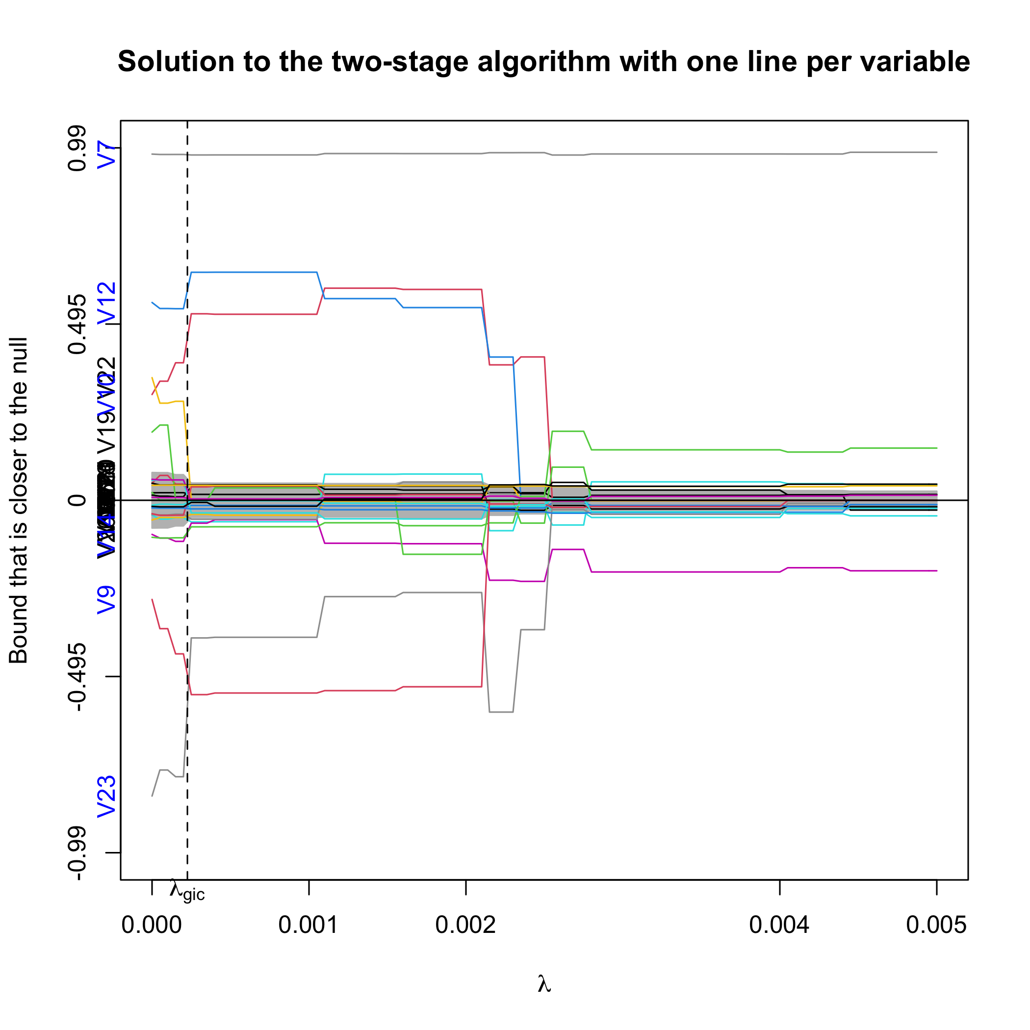
A fast one-stage ProSGPV algorithm is also available when
# run one-stage algorithm
out.sgpv.1 <- pro.sgpv(x = x, y = y, stage = 1)
The selected variables are
out.sgpv.1#> Selected variables are V8 V12 V13 V15 V17 V25 V26coef, summary, and predict
methods are also applicable here.
Moreover, plot function can be used to visualize the
variable selection process for the one-stage algorithm. Point estimates
and 95% confidence intervals are shown for each variable, and the null
bounds are shown in green vertical bars. Selected variables are colored
in blue.
plot(out.sgpv.1)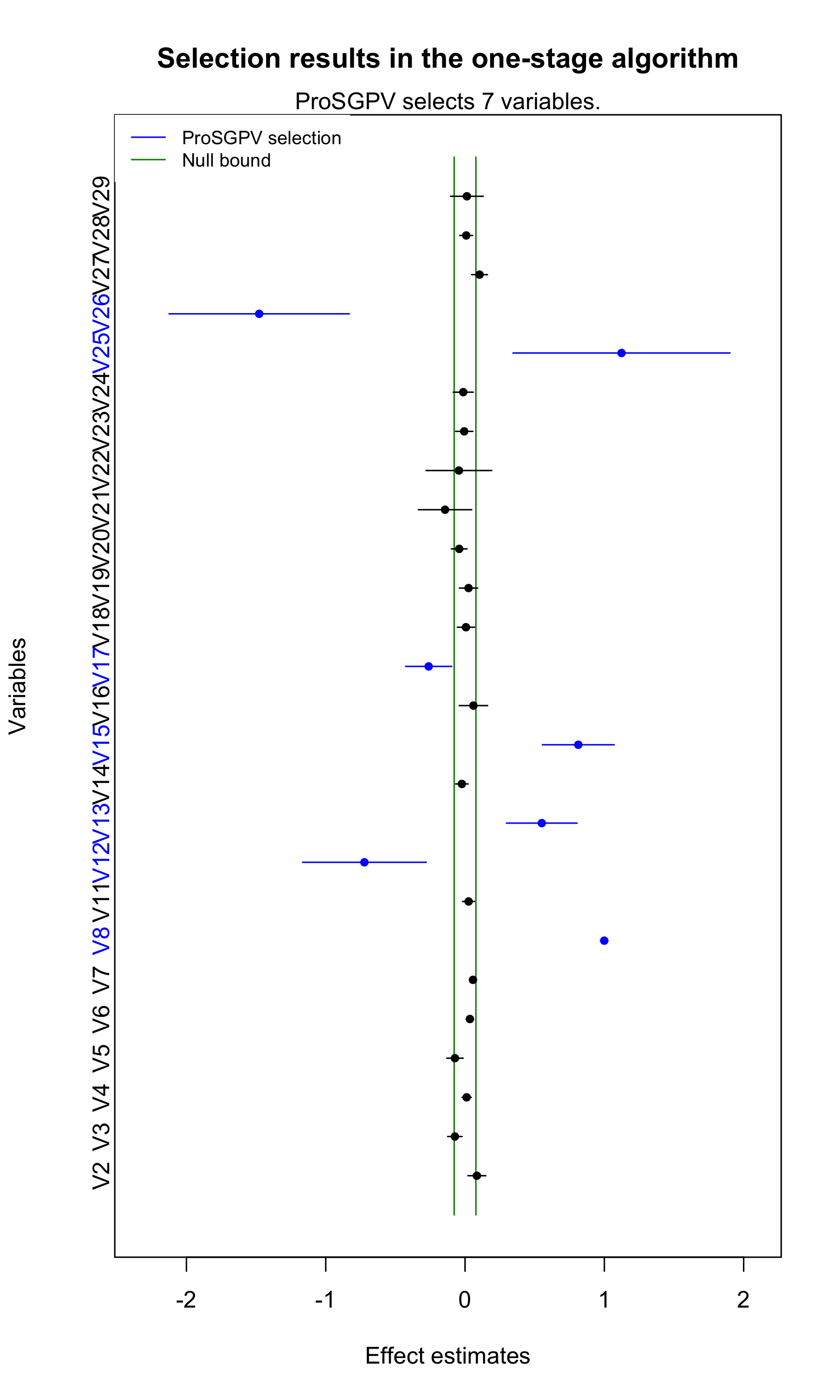
However, it is recommended to use the two-stage algorithm rather than
the one-stage algorithm for better support recovery and parameter
estimation. More importantly, only the two-stage algorithm is available
for high dimensional data where
3.3 More examples
For high-dimensional continuous data examples and GLM and Cox examples, please refer to the vignette folder.
The paper that proposed ProSGPV algorithm in linear regression:
Yi Zuo, Thomas G. Stewart & Jeffrey D. Blume (2021) Variable Selection With Second-Generation P-Values, The American Statistician, DOI: 10.1080/00031305.2021.1946150The paper that proposed ProSGPV algorithm in GLM and Cox models:
Coming soonThe papers regarding the second-generation p-values:
Blume JD, Greevy RA, Welty VF, Smith JR, Dupont WD. An introduction to second-generation p-values. The American Statistician. 2019 Mar 29;73(sup1):157-67.

Blume JD, D’Agostino McGowan L, Dupont WD, Greevy Jr RA. Second-generation p-values: Improved rigor, reproducibility, & transparency in statistical analyses. PLoS One. 2018 Mar 22;13(3):e0188299.
The paper on finding tuning parameters with generalized information criterion:
Fan Y, Tang CY. Tuning parameter selection in high dimensional penalized likelihood. Journal of the Royal Statistical Society: SERIES B: Statistical Methodology. 2013 Jun 1:531-52.