![]()
ROCket was primarily build for ROC curve estimation in the presence of aggregated data. Nevertheless, it can also handle raw samples. In general, aggregating data can be very beneficial when dealing with large datasets. Whenever a dataset consists of categorical or discretized continuous features, the data size can be effectively reduced by calculating sufficient statistics for each constellation of feature values. This saves memory and reduces the time needed to train classification models. Also model accuracy assessment can be done on aggregated data, which yields similar benefits. To this end, ROCket provides functions for ROC curve estimation and AUC calculation.
# From CRAN
install.packages("ROCket")

# From GitHub
# install.packages("devtools")
devtools::install_github("da-zar/ROCket")The easiest way to get started is to prepare a dataset containing all distinct predicted score values together with their count and the number of positive cases. Your dataset could look like this:
nrow(data_agg)
#> [1] 10
head(data_agg)
#>    score totals positives
#> 1:     2  30150     24068
#> 2:     0  62043     24081
#> 3:     1  62863     38730
#> 4:     3   6534      5928
#> 5:    -1  30424      6020
#> 6:    -2   6722       549
You can now pass this data to the rkt_prep function in
order to create an object that will be later used for estimating ROC
curves (possibly with several different algorithms).
prep_data_agg <- rkt_prep(
  scores = data_agg$score,
  positives = data_agg$positives,
  totals = data_agg$totals
)
It is not necessary to use an aggregated dataset. It’s also possible
to have each single observation in a separate row – in this case the
positives argument is the regular indicator (a numeric
vector is required) for positive observations and the
totals argument is not needed anymore (default is 1).
You can print the object, to get some information about the content, or plot it:
prep_data_agg
#> .:: ROCket Prep Object
#> Positives (pos_n): 100000
#> Negatives (neg_n): 100000
#> Pos ECDF (pos_ecdf): rkt_ecdf function
#> Neg ECDF (neg_ecdf): rkt_ecdf function
plot(prep_data_agg)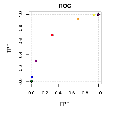
Estimates of the ROC curve can be calculated with the
rkt_roc function. It takes two arguments. The first one is
the rkt_prep object, which contains all the needed data,
and the second one is an integer saying which method of estimation
should be used. A list of implemented methods can be retrieved with the
show_methods function.
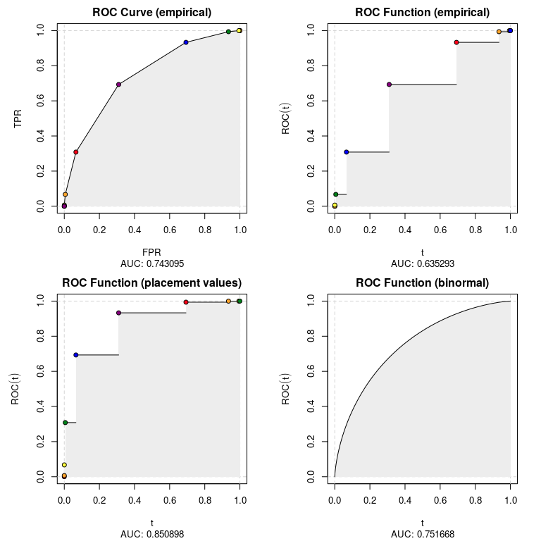
show_methods()
#>    nr                            desc
#> 1:  1           ROC Curve (empirical)
#> 2:  2        ROC Function (empirical)
#> 3:  3 ROC Function (placement values)
#> 4:  4         ROC Function (binormal)
In ROCket, we distinguish two types of ROC curve representations:
In the first case we estimate two functions, the x and y coordinates of the ROC curve (FPR, TPR). These two functions are returned as a list. In the second case the output is a regular function.
Let’s now calculate estimates of the ROC curve using all available methods.
roc_list <- list()
for (i in 1:4){
  roc_list[[i]] <- rkt_roc(prep_data_agg, method = i)
}
The output of rkt_roc can be used to plot the ROC curve
estimates and calculate the AUC.
par(mfrow = c(2, 2))
for (i in 1:4){
  plot(
    roc_list[[i]],
    main = show_methods()[i, desc],
    sub = sprintf('AUC: %f', auc(roc_list[[i]]))
  )
}