The goal of SimCorrMix is to generate continuous (normal, non-normal, or mixture distributions), binary, ordinal, and count (Poisson or Negative Binomial, regular or zero-inflated) variables with a specified correlation matrix, or one continuous variable with a mixture distribution. This package can be used to simulate data sets that mimic real-world clinical or genetic data sets (i.e. plasmodes, as in Vaughan et al., 2009, doi:10.1016/j.csda.2008.02.032). The methods extend those found in the SimMultiCorrData package. Standard normal variables with an imposed intermediate correlation matrix are transformed to generate the desired distributions. Continuous variables are simulated using either Fleishman (1978)’s third-order (doi:10.1007/BF02293811) or Headrick (2002)’s fifth-order (doi:10.1016/S0167-9473(02)00072-5) power method transformation (PMT). Non-mixture distributions require the user to specify mean, variance, skewness, standardized kurtosis, and standardized fifth and sixth cumulants. Mixture distributions require these inputs for the component distributions plus the mixing probabilities. Simulation occurs at the component-level for continuous mixture distributions. The target correlation matrix is specified in terms of correlations with components of continuous mixture variables. These components are transformed into the desired mixture variables using random multinomial variables based on the mixing probabilities. However, the package provides functions to determine expected correlations with continuous mixture variables given target correlations with the components. Binary and ordinal variables are simulated using a modification of GenOrd-package’s ordsample function. Count variables are simulated using the inverse CDF method. There are two simulation pathways which calculate intermediate correlations involving count variables differently. Correlation Method 1 adapts Yahav and Shmueli’s 2012 method (doi:10.1002/asmb.901) and performs best with large count variable means and positive correlations or small means and negative correlations. Correlation Method 2 adapts Barbiero and Ferrari’s 2015 modification of the GenOrd package (doi:10.1002/asmb.2072) and performs best under the opposite scenarios. The optional error loop may be used to improve the accuracy of the final correlation matrix. The package also contains functions to calculate the standardized cumulants of continuous mixture distributions, check parameter inputs, calculate feasible correlation boundaries, and plot simulated variables.
There are several vignettes which accompany this package that may help the user understand the simulation and analysis methods.
Comparison of Correlation Methods 1 and 2
describes the two simulation pathways that can be followed for
generation of correlated data (using corrvar and
corrvar2).
Continuous Mixture Distributions demonstrates
how to simulate one continuous mixture variable using
contmixvar1 and gives a step-by-step guideline for
comparing a simulated distribution to the target distribution.
Expected Cumulants and Correlations for Continuous
Mixture Variables derives the equations used by the function
calc_mixmoments to find the mean, standard deviation, skew,
standardized kurtosis, and standardized fifth and sixth cumulants for a
continuous mixture variable. The vignette also explains how the
functions rho_M1M2 and rho_M1Y calculate the
expected correlations with continuous mixture variables based on the
target correlations with the components.
Overall Workflow for Generation of Correlated Data gives a step-by-step guideline to follow with an example containing continuous non-mixture and mixture, ordinal, zero-inflated Poisson, and zero-inflated Negative Binomial variables. It executes both correlated data simulation functions with and without the error loop.
Variable Types describes the different types of
variables that can be simulated in SimCorrMix, details
the algorithm involved in the optional error loop that helps to minimize
correlation errors, and explains how the feasible correlation boundaries
are calculated for each of the two simulation pathways (using
validcorr and validcorr2).
SimCorrMix can be installed using the following code:
## from GitHub
install.packages("devtools")
devtools::install_github("AFialkowski/SimCorrMix", build_vignettes = TRUE)

## from CRAN
install.packages("SimCorrMix")This is a basic example which shows you how to solve a common problem:
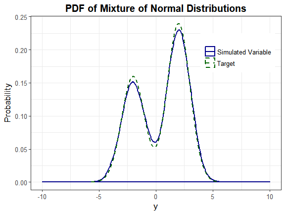
Headrick and Kowalchuk’s steps (2007, doi:10.1080/10629360600605065) to compare the density of a simulated variable to the theoretical density have been modified to accommodate continuous mixture distributions. The component distributions are Normal(-2, 1) and Normal(2, 1). The mixing proportions are 0.4 and 0.6.
The values of
γ1, γ2, γ3,
and γ4 are all 0 for normal variables. The mean and
standard deviation of the mixture variable are found with
calc_mixmoments.
library("SimCorrMix")
#> Loading required package: SimMultiCorrData
#>
#> Attaching package: 'SimMultiCorrData'
#> The following object is masked from 'package:stats':
#>
#>     poly
library("printr")
options(scipen = 999)
n <- 10000
mix_pis <- c(0.4, 0.6)
mix_mus <- c(-2, 2)
mix_sigmas <- c(1, 1)
mix_skews <- rep(0, 2)
mix_skurts <- rep(0, 2)
mix_fifths <- rep(0, 2)
mix_sixths <- rep(0, 2)
Nstcum <- calc_mixmoments(mix_pis, mix_mus, mix_sigmas, mix_skews,
mix_skurts, mix_fifths, mix_sixths)Note that calc_mixmoments returns the standard
deviation, not the variance. The simulation functions require variance
as the input. First, the parameter inputs are checked with
validpar.
validpar(k_mix = 1, method = "Polynomial", means = Nstcum[1],
  vars = Nstcum[2]^2, mix_pis = mix_pis, mix_mus = mix_mus,
  mix_sigmas = mix_sigmas, mix_skews = mix_skews, mix_skurts = mix_skurts,
  mix_fifths = mix_fifths, mix_sixths = mix_sixths)
#> [1] TRUE
Nmix2 <- contmixvar1(n, "Polynomial", Nstcum[1], Nstcum[2]^2, mix_pis, mix_mus,
  mix_sigmas, mix_skews, mix_skurts, mix_fifths, mix_sixths)
#> Total Simulation time: 0.002 minutes
Look at a summary of the target distribution and compare to a summary of the simulated distribution.
SumN <- summary_var(Y_comp = Nmix2$Y_comp, Y_mix = Nmix2$Y_mix,
  means = Nstcum[1], vars = Nstcum[2]^2, mix_pis = mix_pis, mix_mus = mix_mus,
  mix_sigmas = mix_sigmas, mix_skews = mix_skews, mix_skurts = mix_skurts,
  mix_fifths = mix_fifths, mix_sixths = mix_sixths)
knitr::kable(SumN$target_mix, digits = 5, row.names = FALSE,
caption = "Summary of Target Distribution")| Distribution | Mean | SD | Skew | Skurtosis | Fifth | Sixth |
|---|---|---|---|---|---|---|
| 1 | 0.4 | 2.2 | -0.2885 | -1.15402 | 1.79302 | 6.17327 |
knitr::kable(SumN$mix_sum, digits = 5, row.names = FALSE,
caption = "Summary of Simulated Distribution")| Distribution | N | Mean | SD | Median | Min | Max | Skew | Skurtosis | Fifth | Sixth |
|---|---|---|---|---|---|---|---|---|---|---|
| 1 | 10000 | 0.4 | 2.19989 | 1.05078 | -5.69433 | 5.341 | -0.2996 | -1.15847 | 1.84723 | 6.1398 |
Nmix2$constants| c0 | c1 | c2 | c3 | c4 | c5 |
|---|---|---|---|---|---|
| 0 | 1 | 0 | 0 | 0 | 0 |
| 0 | 1 | 0 | 0 | 0 | 0 |
Nmix2$valid.pdf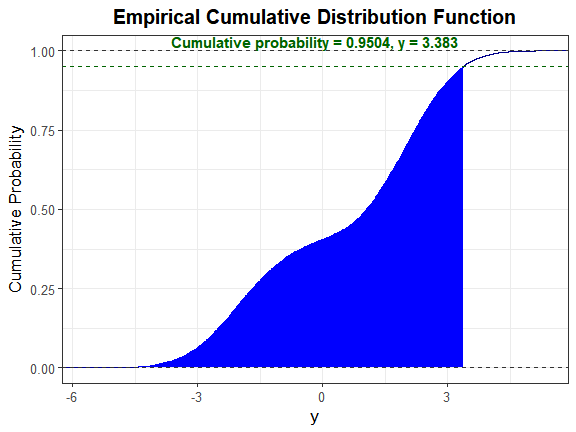
#> [1] "TRUE" "TRUE"Let α = 0.05. Since there are no quantile functions for
mixture distributions, determine where the cumulative probability equals
1 − α = 0.95. The boundaries for uniroot were
determined through trial and error.
fx <- function(x) 0.4 * dnorm(x, -2, 1) + 0.6 * dnorm(x, 2, 1)
cfx <- function(x, alpha, FUN = fx) {
  integrate(function(x, FUN = fx) FUN(x), -Inf, x, subdivisions = 1000,
    stop.on.error = FALSE)$value - (1 - alpha)
}
y_star <- uniroot(cfx, c(3.3, 3.4), tol = 0.001, alpha = 0.05)$root
y_star
#> [1] 3.382993We will use the function SimMultiCorrData::sim_cdf_prob
to determine the cumulative probability for Y up to
y_star. This function is based on Martin Maechler’s
ecdf function [@Stats].
sim_cdf_prob(sim_y = Nmix2$Y_mix[, 1], delta = y_star)$cumulative_prob
#> [1] 0.9504
This is approximately equal to the 1 − α value of 0.95, indicating the method provides a good approximation to the actual distribution.
plot_simpdf_theory(sim_y = Nmix2$Y_mix[, 1], ylower = -10, yupper = 10,
  title = "PDF of Mixture of Normal Distributions", fx = fx, lower = -Inf,
  upper = Inf)
We can also plot the empirical cdf and show the cumulative probability up to y_star.
plot_sim_cdf(sim_y = Nmix2$Y_mix[, 1], calc_cprob = TRUE, delta = y_star)