
![]()

Designed to be a tidy API wrapper for the Bureau of Labor Statistics (BLS.) The package has additional functions to help parse, analyze and visualize the data. The package utilizes “tidyverse” concepts for internal functionality and encourages the use of those concepts with the output data.
install.packages("blscrapeR")devtools::install_github("keberwein/blscrapeR")Before getting started, you’ll probably want to head over to the BLS and get set up with an API key. While an API key is not required to use the package, the query limits are much higher if you have a key and you’ll have access to more data. Plus, it’s free (as in beer), so why not?
For “quick and dirty” type of analysis, the package has some quick functions that will pull metrics from the API without series numbers. These include:
quick_unemp_rate(): Official Unemployment Rate
(U-3)quick_unemp_level(): Unemployment Levelquick_employed_rate(): Employment-Population Ratioquick_employed_level(): Employment Levelquick_laborForce_rate(): Labor Force Participation
Ratequick_laborForce_level(): Civilian Labor Force
Levelquick_nonfarm_employed(): Total Nonfarm Payroll
Employmentlibrary(blscrapeR)
# Grab the Unemployment Rate (U-3)
df <- quick_unemp_rate()
head(df, 5)
#> # A tibble: 5 x 6
#> year period periodName value footnotes seriesID
#> <dbl> <list> <list> <dbl> <list> <list>
#> 1 2017 <chr [1]> <chr [1]> 4.1 <chr [1]> <chr [1]>
#> 2 2017 <chr [1]> <chr [1]> 4.2 <chr [1]> <chr [1]>
#> 3 2017 <chr [1]> <chr [1]> 4.4 <chr [1]> <chr [1]>
#> 4 2017 <chr [1]> <chr [1]> 4.3 <chr [1]> <chr [1]>
#> 5 2017 <chr [1]> <chr [1]> 4.4 <chr [1]> <chr [1]>Some knowledge of BLS ids are needed to query the API. The package
includes a “fuzzy search” function to help find these ids. There are
currently more than 75,000 series ids in the package’s internal data
set, series_ids. While these aren’t all the series ids the
BLS offers, it contains the most popular. The BLS Data Finder is another
good resource for finding series ids, that may not be in the internal
data set.
library(blscrapeR)
# Find series ids relating to the total labor force in LA.
ids <- search_ids(keyword = c("Labor Force", "Los Angeles"))
head(ids)
#> # A tibble: 6 x 4
#>                                                                  series_title
#>                                                                         <chr>
#> 1 Labor Force: Balance Of California, State Less Los Angeles-Long Beach-Glend
#> 2  Labor Force: Los Angeles-Long Beach-Glendale, Ca Metropolitan Division (S)
#> 3 Labor Force: Balance Of California, State Less Los Angeles-Long Beach-Glend
#> 4       Labor Force: Los Angeles-Long Beach, Ca Combined Statistical Area (U)
#> 5                                     Labor Force: Los Angeles County, Ca (U)
#> 6                                       Labor Force: Los Angeles City, Ca (U)
#> # ... with 3 more variables: series_id <chr>, seasonal <chr>,
#> # periodicity_code <chr>library(blscrapeR)
# Find series ids relating to median weekly earnings of women software developers.
ids <- search_ids(keyword = c("Earnings", "Software", "Women"))
head(ids)
#> # A tibble: 1 x 4
#> series_title
#> <chr>
#> 1 (Unadj)- Median Usual Weekly Earnings (Second Quartile), Employed Full Time
#> # ... with 3 more variables: series_id <chr>, seasonal <chr>,
#> # periodicity_code <chr>When working with local data, it’s often necessary to use Federal Information Processing Series (FIPS) codes to identify specific regions. The package includes a helper function to list county FIPS codes for a given state.
library(blscrapeR)
# Get a list of all county FIPS codes for Florida.
fl_fips <- county_fips(state = "FL")
head(fl_fips)
#> # A tibble: 6 x 3
#>   fips_state fips_county county_name
#>   <chr>      <chr>       <chr>
#> 1 12         001         Alachua
#> 2 12         003         Baker
#> 3 12         005         Bay
#> 4 12         007         Bradford
#> 5 12         009         Brevard
#> 6 12 011 Broward You should consider getting an API key
form the BLS. The package has a function to install your key in your
.Renviron so you’ll only have to worry about it once. Plus,
it will add extra security by not having your key hard-coded in your
scripts for all the world to see.
| Service | Version 2.0 (Registered) | Version 1.0 (Unregistered) |
|---|---|---|
| Daily query limit | 500 | 25 |
| Series per query limit | 50 | 25 |
| Years per query limit | 20 | 10 |
| Net/Percent Changes | Yes | No |
| Optional annual averages | Yes | No |
| Series descriptions | Yes | No |
library(blscrapeR)

# Grab several data sets from the BLS at onece.
# NOTE on series IDs:
# EMPLOYMENT LEVEL - Civilian labor force - LNS12000000
# UNEMPLOYMENT LEVEL - Civilian labor force - LNS13000000
# UNEMPLOYMENT RATE - Civilian labor force - LNS14000000
df <- bls_api(c("LNS12000000", "LNS13000000", "LNS14000000"),
              startyear = 2008, endyear = 2017, Sys.getenv("BLS_KEY")) %>%
    # Add time-series dates
dateCast()Registered users (with an API key) can request additional calculations, annual averages, and catalog descriptions.
library(blscrapeR)
# Request data with year-over-year calculations and annual averages.
df <- bls_api(c("LNS14000000"),
              startyear = 2010, endyear = 2020,
              registrationKey = "BLS_KEY",
              calculations = TRUE, annualaverage = TRUE, catalog = TRUE)
head(df)
Tip: If you have set your API key in your
.Renviron using set_bls_key(), you can simply
pass the string "BLS_KEY" as the
registrationKey argument to automatically use it.
# Plot employment level
library(ggplot2)
gg1200 <- subset(df, seriesID=="LNS12000000")
library(ggplot2)
ggplot(gg1200, aes(x=date, y=value)) +
    geom_line() +
    labs(title = "Employment Level - Civ. Labor Force")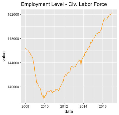
library(blscrapeR)
library(tidyverse)
# Median Usual Weekly Earnings by Occupation, Unadjusted Second Quartile.
# In current dollars
df <- bls_api(c("LEU0254530800", "LEU0254530600"), startyear = 2000, endyear = 2016, registrationKey = Sys.getenv("BLS_KEY")) %>%
    pivot_wider(names_from = seriesID, values_from = value) %>% dateCast()
# A little help from ggplot2!
library(ggplot2)
ggplot(data = df, aes(x = date)) +
geom_line(aes(y = LEU0254530800, color = "Database Admins.")) +
geom_line(aes(y = LEU0254530600, color = "Software Devs.")) +
labs(title = "Median Weekly Earnings by Occupation") + ylab("value") +
theme(legend.position="top", plot.title = element_text(hjust = 0.5)) 
For more advanced usage, please see the package vignettes.
Although there are many measures of inflation, the CPI’s “Consumer Price Index for All Urban Consumers: All Items” is normally the headline inflation rate one would hear about on the news (see FRED).
Getting these data from the blscrapeR package is easy
enough:
{r eval=FALSE} library(blscrapeR) df <- bls_api("CUSR0000SA0") head(df)
Due to the limitations of the API, we are only able to gather twenty years of data per request. However the formula for calculating inflation is based on the 1980 dollar, so the data from the API aren’t sufficient.
The package includes a function that collects information form the CPI beginning at 1947 and calculates inflation.
To find out the value of a January 2015 dollar in January 2023, we
just make a simple function call. Looking at the
adj_dollar_value column. We can see that the value of a
2015 dollar in 2023 was approximately $1.32.
```{r eval=FALSE} df <- inflation_adjust(“2015-01-01”) %>% arrange(desc(date)) head(df)
library(blscrapeR) # A tibble: 6 × 7 date period year value base_date
adj_dollar_value month_ovr_month_pct_change
If we want to check our results, we can head over to the CPI [Inflation Calculator](https://data.bls.gov/cgi-bin/cpicalc.pl) on the BLS website.


### Annual Inflation Percentage Increase

```{r eval=FALSE}
library(blscrapeR)
library(ggplot2)

ggplot(data = df, aes(x = date)) +
    geom_line(aes(y = adj_dollar_value, color = "2015 Adjusted Dollar Value")) +
    labs(title = "Inflation Since 2015") + ylab("2015 Adjusted Dollar Value") +
    theme(legend.position="top", plot.title = element_text(hjust = 0.5))


ggplot(data = df, aes(x = date)) +
    geom_line(aes(y = month_ovr_month_pct_change, color = "MoM Pct Change")) +
    labs(title = "Month over Month Inflation Pct Change") + ylab("MoM Pct Change") +
    theme(legend.position="top", plot.title = element_text(hjust = 0.5))


Another typical use of the CPI is to determine price escalation. This is especially common in escalation contracts. While there are many different ways one could calculate escalation below is a simple example. Note: the BLS recommends using non-seasonally adjusted data for escalation calculations.
Suppose we want the price escalation of $100 investment we made in January 2014 to February 2015:
Disclaimer: Escalation is normally formulated by lawyers and bankers, the author(s) of this package are neither, so the above should only be considered a code example.
```{r eval=FALSE} library(blscrapeR) library(dplyr) df <- bls_api(“CUSR0000SA0”, startyear = 2014, endyear = 2015) head(df)
year period periodName value footnotes seriesID
1 2015 M12 December 238. “” CUSR0000SA0 2 2015 M11 November 238. “”
CUSR0000SA0 3 2015 M10 October 238. “” CUSR0000SA0 4 2015 M09 September
237. “” CUSR0000SA0 5 2015 M08 August 238. “” CUSR0000SA0 6 2015 M07
July 238. “” CUSR0000SA0
base_value <- 100
base_cpi <- subset(df, year==2014 & periodName==“January”, select = “value”)
new_cpi <- subset(df, year==2015 & periodName==“February”, select = “value”)
round((base_value / base_cpi) * new_cpi, 2) value 1 100.02
```