
![]()
![]()
![]()
![]()
brglm2 provides tools for the estimation and inference from generalized linear models using various methods for bias reduction. brglm2 supports all generalized linear models supported in R, and provides methods for multinomial logistic regression (nominal responses), adjacent category models (ordinal responses), and negative binomial regression (for potentially overdispered count responses).
Reduction of estimation bias is achieved by solving either the mean-bias reducing adjusted score equations in Firth (1993) and Kosmidis & Firth (2009) or the median-bias reducing adjusted score equations in Kenne et al (2017), or through the direct subtraction of an estimate of the bias of the maximum likelihood estimator from the maximum likelihood estimates as prescribed in Cordeiro and McCullagh (1991). Kosmidis et al (2020) provides a unifying framework and algorithms for mean and median bias reduction for the estimation of generalized linear models.
In the special case of generalized linear models for binomial and multinomial responses (both ordinal and nominal), the adjusted score equations return estimates with improved frequentist properties, that are also always finite, even in cases where the maximum likelihood estimates are infinite (e.g. complete and quasi-complete separation). See, Kosmidis & Firth (2021) for the proof of the latter result in the case of mean bias reduction for logistic regression (and, for more general binomial-response models where the likelihood is penalized by a power of the Jeffreys’ invariant prior).
For logistic regression, brglm2 also provides methods for maximum Diaconis-Ylvisaker prior penalized likelihood (MDYPL) estimation, and corresponding methods for high-dimensionality corrections of the aggregate bias of the estimator and the usual statistics used for inference; see Sterzinger and Kosmidis, 2024.
The core model fitters are implemented by the functions
brglm_fit() (univariate generalized linear models) and
mdyplFit() (logistic regression), and
brmultinom() (baseline category logit models for nominal
multinomial responses), bracl() (adjacent category logit
models for ordinal multinomial responses), and brnb()
(negative binomial regression).
Install the current version from CRAN:
install.packages("brglm2")or the development version from github:
# install.packages("remotes")
remotes::install_github("ikosmidis/brglm2", ref = "develop")Below we follow the example of Heinze and Schemper (2002)
and fit a logistic regression model using maximum likelihood (ML) to
analyze data from a study on endometrial cancer (see
?brglm2::endometrial for details and references).
library("brglm2")
data("endometrial", package = "brglm2")
modML <- glm(HG ~ NV + PI + EH, family = binomial("logit"), data = endometrial)
summary(modML)
#>
#> Call:
#> glm(formula = HG ~ NV + PI + EH, family = binomial("logit"),
#>     data = endometrial)
#>
#> Coefficients:
#>               Estimate Std. Error z value Pr(>|z|)
#> (Intercept)    4.30452    1.63730   2.629 0.008563 **
#> NV            18.18556 1715.75089   0.011 0.991543
#> PI            -0.04218    0.04433  -0.952 0.341333
#> EH            -2.90261    0.84555  -3.433 0.000597 ***
#> ---
#> Signif. codes:  0 '***' 0.001 '**' 0.01 '*' 0.05 '.' 0.1 ' ' 1
#>
#> (Dispersion parameter for binomial family taken to be 1)
#>
#>     Null deviance: 104.903  on 78  degrees of freedom
#> Residual deviance:  55.393  on 75  degrees of freedom
#> AIC: 63.393
#>
#> Number of Fisher Scoring iterations: 17
The ML estimate of the parameter for NV is actually
infinite, as can be quickly verified using the detectseparation
R package
# install.packages("detectseparation")
library("detectseparation")
#>
#> Attaching package: 'detectseparation'
#> The following objects are masked from 'package:brglm2':
#>
#>     check_infinite_estimates, detect_separation
update(modML, method = detect_separation)
#> Implementation: ROI | Solver: lpsolve
#> Separation: TRUE
#> Existence of maximum likelihood estimates
#> (Intercept)          NV          PI          EH
#>           0         Inf           0           0
#> 0: finite value, Inf: infinity, -Inf: -infinity
The reported, apparently finite estimate
r round(coef(summary(modML))["NV", "Estimate"], 3) for
NV is merely due to false convergence of the iterative
estimation procedure for ML. The same is true for the estimated standard
error, and, hence the value 0.011 for the z-statistic cannot be
trusted for inference on the effect size for NV.
As mentioned earlier, many of the estimation methods implemented in brglm2 not only return estimates with improved frequentist properties (e.g. asymptotically smaller mean and median bias than what ML typically delivers), but also estimates and estimated standard errors that are always finite in binomial (e.g. logistic, probit, and complementary log-log regression) and multinomial regression models (e.g. baseline category logit models for nominal responses, and adjacent category logit models for ordinal responses). For example, the code chunk below refits the model on the endometrial cancer study data using mean bias reduction.
summary(update(modML, method = "brglm_fit"))
#>
#> Call:
#> glm(formula = HG ~ NV + PI + EH, family = binomial("logit"),
#>     data = endometrial, method = "brglm_fit")
#>
#> Deviance Residuals:
#>     Min       1Q   Median       3Q      Max
#> -1.4740  -0.6706  -0.3411   0.3252   2.6123
#>
#> Coefficients:
#>             Estimate Std. Error z value Pr(>|z|)
#> (Intercept)  3.77456    1.48869   2.535 0.011229 *
#> NV           2.92927    1.55076   1.889 0.058902 .
#> PI          -0.03475    0.03958  -0.878 0.379915
#> EH          -2.60416    0.77602  -3.356 0.000791 ***
#> ---
#> Signif. codes:  0 '***' 0.001 '**' 0.01 '*' 0.05 '.' 0.1 ' ' 1
#>
#> (Dispersion parameter for binomial family taken to be 1)
#>
#>     Null deviance: 104.903  on 78  degrees of freedom
#> Residual deviance:  56.575  on 75  degrees of freedom
#> AIC:  64.575
#>
#> Type of estimator: AS_mixed (mixed bias-reducing adjusted score equations)
#> Number of Fisher Scoring iterations: 6
A quick comparison of the output from mean bias reduction to that
from ML reveals a dramatic change in the z-statistic for
NV, now that estimates and estimated standard errors are
finite. In particular, the evidence against the null of NV
not contributing to the model in the presence of the other covariates
being now stronger.
See ?brglm_fit and ?brglm_control for more
examples and the other estimation methods for generalized linear models,
including median bias reduction and maximum penalized likelihood with
Jeffreys’ prior penalty. Also do not forget to take a look at the
vignettes (vignette(package = "brglm2")) for details and
more case studies.
See, also ?expo for a method to estimate the exponential
of regression parameters, such as odds ratios from logistic regression
models, while controlling for other covariate information. Estimation
can be performed using maximum likelihood or various estimators with
smaller asymptotic mean and median bias, that are also guaranteed to be
finite, even if the corresponding maximum likelihood estimates are
infinite. For example, modML is a logistic regression fit,
so the exponential of each coefficient is an odds ratio while
controlling for other covariates. To estimate those odds ratios using
the correction* method for mean bias reduction (see
?expo for details) we do
expoRB <- expo(modML, type = "correction*")
expoRB
#>
#> Call:
#> expo.glm(object = modML, type = "correction*")
#>
#> Odds ratios
#>              Estimate Std. Error     2.5 %  97.5 %
#> (Intercept) 20.671820  33.136501  0.893141 478.451
#> NV           8.496974   7.825239  1.397511  51.662
#> PI           0.965089   0.036795  0.895602   1.040
#> EH           0.056848   0.056344  0.008148   0.397
#>
#>
#> Type of estimator: correction* (explicit mean bias correction with a multiplicative adjustment)
The odds ratio between presence of neovasculation and high histology
grade (HG) is estimated to be 8.497, while controlling for
PI and EH. So, for each value of PI and EH,
the estimated odds of high histology grade are about 8.5 times higher
when neovasculation is present. An approximate 95% interval for the
latter odds ratio is (1.4, 51.7) providing evidence of association
between NV and HG while controlling for
PI and EH. Note here that, the maximum
likelihood estimate of the odds ratio is not as useful as the
correction* estimate, because it is +∞ with an infinite
standard error (see previous section).
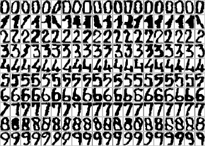
Consider the Multiple
Features dataset, which consists of digits (0-9) extracted from a
collection of maps from a Dutch public utility. Two hundred
30 × 48 binary images per digit were available, which have
then been used to extract feature sets. The digits are shown below using
pixel averages in 2 x 3 windows.
data("MultipleFeatures", package = "brglm2")
par(mfrow = c(10, 20), mar = numeric(4) + 0.1)
for (c_digit in 0:9) {
    df <- subset(MultipleFeatures, digit == c_digit)
    df <- as.matrix(df[, paste("pix", 1:240, sep = ".")])
    for (inst in 1:20) {
        m <- matrix(df[inst, ], 15, 16)[, 16:1]
        image(m, col = grey.colors(7, 1, 0), xaxt = "n", yaxt = "n")
    }
}
We focus on the setting of Sterzinger and Kosmidis (2024,
Section 8) on explaining the character shapes of the digit
7 in terms of 76 Fourier coefficients (fou
features), which are computed to be rotationally invariant, and 64
Karhunen-Loève coefficients (kar features), using 1000
randomly selected digits. Depending on the font, the level of noise
introduced during digitization, and the downscaling of the digits to
binary images, difficulties may arise in discriminating instances of the
digit 7 to instances of the digits 1 and
4. Also, if only rotation invariant features, like
fou, are used difficulties may arise in discriminating
instances of the digit 7 to instances of the digit
2.
The data is perfectly separated for both the model with only
fou features, and the model with fou and
kar features, and the maximized likelihood is zero for both
models.
## Center the fou.* and kar.* features
vars <- grep("fou|kar", names(MultipleFeatures), value = TRUE)
train_id <- which(MultipleFeatures$training)
MultipleFeatures[train_id, vars] <- scale(MultipleFeatures[train_id, vars], scale = FALSE)
## Set up module formulas
full_fm <- formula(paste("I(digit == 7) ~", paste(vars, collapse = " + ")))
nest_vars <- grep("fou", vars, value = TRUE)
nest_fm <- formula(paste("I(digit == 7) ~", paste(nest_vars, collapse = " + ")))
## Fit the models using maximum likelihood
full_sep <- glm(full_fm, data = MultipleFeatures, family = binomial(), subset = training,
                method = detect_separation)
nest_sep <- update(full_sep, nest_fm)
full_sep$outcome
#> [1] TRUE
nest_sep$outcome
#> [1] TRUE
As a result, the likelihood ratio statistic comparing the two models
will be trivially zero, regardless of any evidence against the
hypothesis that the model with only fou features is an as
good description of 7 as the model with both
fou and kar features.
anova(update(nest_sep, method = glm.fit),
      update(full_sep, method = glm.fit))
#> Warning: glm.fit: algorithm did not converge
#> Warning: glm.fit: fitted probabilities numerically 0 or 1 occurred
#> Warning: glm.fit: algorithm did not converge
#> Warning: glm.fit: fitted probabilities numerically 0 or 1 occurred
#> Analysis of Deviance Table
#>
#> Model 1: I(digit == 7) ~ fou.1 + fou.2 + fou.3 + fou.4 + fou.5 + fou.6 +
#>     fou.7 + fou.8 + fou.9 + fou.10 + fou.11 + fou.12 + fou.13 +
#>     fou.14 + fou.15 + fou.16 + fou.17 + fou.18 + fou.19 + fou.20 +
#>     fou.21 + fou.22 + fou.23 + fou.24 + fou.25 + fou.26 + fou.27 +
#>     fou.28 + fou.29 + fou.30 + fou.31 + fou.32 + fou.33 + fou.34 +
#>     fou.35 + fou.36 + fou.37 + fou.38 + fou.39 + fou.40 + fou.41 +
#>     fou.42 + fou.43 + fou.44 + fou.45 + fou.46 + fou.47 + fou.48 +
#>     fou.49 + fou.50 + fou.51 + fou.52 + fou.53 + fou.54 + fou.55 +
#>     fou.56 + fou.57 + fou.58 + fou.59 + fou.60 + fou.61 + fou.62 +
#>     fou.63 + fou.64 + fou.65 + fou.66 + fou.67 + fou.68 + fou.69 +
#>     fou.70 + fou.71 + fou.72 + fou.73 + fou.74 + fou.75 + fou.76
#> Model 2: I(digit == 7) ~ fou.1 + fou.2 + fou.3 + fou.4 + fou.5 + fou.6 +
#>     fou.7 + fou.8 + fou.9 + fou.10 + fou.11 + fou.12 + fou.13 +
#>     fou.14 + fou.15 + fou.16 + fou.17 + fou.18 + fou.19 + fou.20 +
#>     fou.21 + fou.22 + fou.23 + fou.24 + fou.25 + fou.26 + fou.27 +
#>     fou.28 + fou.29 + fou.30 + fou.31 + fou.32 + fou.33 + fou.34 +
#>     fou.35 + fou.36 + fou.37 + fou.38 + fou.39 + fou.40 + fou.41 +
#>     fou.42 + fou.43 + fou.44 + fou.45 + fou.46 + fou.47 + fou.48 +
#>     fou.49 + fou.50 + fou.51 + fou.52 + fou.53 + fou.54 + fou.55 +
#>     fou.56 + fou.57 + fou.58 + fou.59 + fou.60 + fou.61 + fou.62 +
#>     fou.63 + fou.64 + fou.65 + fou.66 + fou.67 + fou.68 + fou.69 +
#>     fou.70 + fou.71 + fou.72 + fou.73 + fou.74 + fou.75 + fou.76 +
#>     kar.1 + kar.2 + kar.3 + kar.4 + kar.5 + kar.6 + kar.7 + kar.8 +
#>     kar.9 + kar.10 + kar.11 + kar.12 + kar.13 + kar.14 + kar.15 +
#>     kar.16 + kar.17 + kar.18 + kar.19 + kar.20 + kar.21 + kar.22 +
#>     kar.23 + kar.24 + kar.25 + kar.26 + kar.27 + kar.28 + kar.29 +
#>     kar.30 + kar.31 + kar.32 + kar.33 + kar.34 + kar.35 + kar.36 +
#>     kar.37 + kar.38 + kar.39 + kar.40 + kar.41 + kar.42 + kar.43 +
#>     kar.44 + kar.45 + kar.46 + kar.47 + kar.48 + kar.49 + kar.50 +
#>     kar.51 + kar.52 + kar.53 + kar.54 + kar.55 + kar.56 + kar.57 +
#>     kar.58 + kar.59 + kar.60 + kar.61 + kar.62 + kar.63 + kar.64
#>   Resid. Df Resid. Dev Df   Deviance Pr(>Chi)
#> 1       923 3.1661e-07
#> 2       859 1.6140e-08 64 3.0047e-07        1
Let’s fit the models using maximum Diaconis-Ylvisaker prior penalized
likelihood (MDYPL) with a shrinkage parameter alpha in
(0, 1), which always results in finite estimates; see
?brglm2::mdypl_fit. The corresponding penalized likelihood
ratio test (see ?brglm2::plrtest and
?brglm2::summary.mdyplFit) results again in no evidence
against the hypothesis.
full_m <- update(full_sep, method = mdypl_fit)
nest_m <- update(nest_sep, method = mdypl_fit, alpha = full_m$alpha)
plrtest(nest_m, full_m)
#> Analysis of Deviance Table
#>
#> Model 1: I(digit == 7) ~ fou.1 + fou.2 + fou.3 + fou.4 + fou.5 + fou.6 +
#>     fou.7 + fou.8 + fou.9 + fou.10 + fou.11 + fou.12 + fou.13 +
#>     fou.14 + fou.15 + fou.16 + fou.17 + fou.18 + fou.19 + fou.20 +
#>     fou.21 + fou.22 + fou.23 + fou.24 + fou.25 + fou.26 + fou.27 +
#>     fou.28 + fou.29 + fou.30 + fou.31 + fou.32 + fou.33 + fou.34 +
#>     fou.35 + fou.36 + fou.37 + fou.38 + fou.39 + fou.40 + fou.41 +
#>     fou.42 + fou.43 + fou.44 + fou.45 + fou.46 + fou.47 + fou.48 +
#>     fou.49 + fou.50 + fou.51 + fou.52 + fou.53 + fou.54 + fou.55 +
#>     fou.56 + fou.57 + fou.58 + fou.59 + fou.60 + fou.61 + fou.62 +
#>     fou.63 + fou.64 + fou.65 + fou.66 + fou.67 + fou.68 + fou.69 +
#>     fou.70 + fou.71 + fou.72 + fou.73 + fou.74 + fou.75 + fou.76
#> Model 2: I(digit == 7) ~ fou.1 + fou.2 + fou.3 + fou.4 + fou.5 + fou.6 +
#>     fou.7 + fou.8 + fou.9 + fou.10 + fou.11 + fou.12 + fou.13 +
#>     fou.14 + fou.15 + fou.16 + fou.17 + fou.18 + fou.19 + fou.20 +
#>     fou.21 + fou.22 + fou.23 + fou.24 + fou.25 + fou.26 + fou.27 +
#>     fou.28 + fou.29 + fou.30 + fou.31 + fou.32 + fou.33 + fou.34 +
#>     fou.35 + fou.36 + fou.37 + fou.38 + fou.39 + fou.40 + fou.41 +
#>     fou.42 + fou.43 + fou.44 + fou.45 + fou.46 + fou.47 + fou.48 +
#>     fou.49 + fou.50 + fou.51 + fou.52 + fou.53 + fou.54 + fou.55 +
#>     fou.56 + fou.57 + fou.58 + fou.59 + fou.60 + fou.61 + fou.62 +
#>     fou.63 + fou.64 + fou.65 + fou.66 + fou.67 + fou.68 + fou.69 +
#>     fou.70 + fou.71 + fou.72 + fou.73 + fou.74 + fou.75 + fou.76 +
#>     kar.1 + kar.2 + kar.3 + kar.4 + kar.5 + kar.6 + kar.7 + kar.8 +
#>     kar.9 + kar.10 + kar.11 + kar.12 + kar.13 + kar.14 + kar.15 +
#>     kar.16 + kar.17 + kar.18 + kar.19 + kar.20 + kar.21 + kar.22 +
#>     kar.23 + kar.24 + kar.25 + kar.26 + kar.27 + kar.28 + kar.29 +
#>     kar.30 + kar.31 + kar.32 + kar.33 + kar.34 + kar.35 + kar.36 +
#>     kar.37 + kar.38 + kar.39 + kar.40 + kar.41 + kar.42 + kar.43 +
#>     kar.44 + kar.45 + kar.46 + kar.47 + kar.48 + kar.49 + kar.50 +
#>     kar.51 + kar.52 + kar.53 + kar.54 + kar.55 + kar.56 + kar.57 +
#>     kar.58 + kar.59 + kar.60 + kar.61 + kar.62 + kar.63 + kar.64
#>   Resid. Df Resid. Dev Df Deviance Pr(>Chi)
#> 1       923     97.305
#> 2       859     32.945 64   64.359   0.4639
Nevertheless, full_m involves 141 parameters, which is
relatively large compared to the 1000 available observations. The
distribution of the penalized likelihood ratio statistic may be far from
the asymptotic χ2 distribution that we expect under
usual asymptotics.
In stark contrast to the evidence quantified by the previous tests,
the high-dimensionality correction to the penalized likelihood ratio
statistic under proportional asymptotics proposed in Sterzinger and Kosmidis
(2024) results in strong evidence against the model with
fou features only.
plrtest(nest_m, full_m, hd_correction = TRUE)
#> Analysis of Deviance Table
#>
#> Model 1: I(digit == 7) ~ fou.1 + fou.2 + fou.3 + fou.4 + fou.5 + fou.6 +
#>     fou.7 + fou.8 + fou.9 + fou.10 + fou.11 + fou.12 + fou.13 +
#>     fou.14 + fou.15 + fou.16 + fou.17 + fou.18 + fou.19 + fou.20 +
#>     fou.21 + fou.22 + fou.23 + fou.24 + fou.25 + fou.26 + fou.27 +
#>     fou.28 + fou.29 + fou.30 + fou.31 + fou.32 + fou.33 + fou.34 +
#>     fou.35 + fou.36 + fou.37 + fou.38 + fou.39 + fou.40 + fou.41 +
#>     fou.42 + fou.43 + fou.44 + fou.45 + fou.46 + fou.47 + fou.48 +
#>     fou.49 + fou.50 + fou.51 + fou.52 + fou.53 + fou.54 + fou.55 +
#>     fou.56 + fou.57 + fou.58 + fou.59 + fou.60 + fou.61 + fou.62 +
#>     fou.63 + fou.64 + fou.65 + fou.66 + fou.67 + fou.68 + fou.69 +
#>     fou.70 + fou.71 + fou.72 + fou.73 + fou.74 + fou.75 + fou.76
#> Model 2: I(digit == 7) ~ fou.1 + fou.2 + fou.3 + fou.4 + fou.5 + fou.6 +
#>     fou.7 + fou.8 + fou.9 + fou.10 + fou.11 + fou.12 + fou.13 +
#>     fou.14 + fou.15 + fou.16 + fou.17 + fou.18 + fou.19 + fou.20 +
#>     fou.21 + fou.22 + fou.23 + fou.24 + fou.25 + fou.26 + fou.27 +
#>     fou.28 + fou.29 + fou.30 + fou.31 + fou.32 + fou.33 + fou.34 +
#>     fou.35 + fou.36 + fou.37 + fou.38 + fou.39 + fou.40 + fou.41 +
#>     fou.42 + fou.43 + fou.44 + fou.45 + fou.46 + fou.47 + fou.48 +
#>     fou.49 + fou.50 + fou.51 + fou.52 + fou.53 + fou.54 + fou.55 +
#>     fou.56 + fou.57 + fou.58 + fou.59 + fou.60 + fou.61 + fou.62 +
#>     fou.63 + fou.64 + fou.65 + fou.66 + fou.67 + fou.68 + fou.69 +
#>     fou.70 + fou.71 + fou.72 + fou.73 + fou.74 + fou.75 + fou.76 +
#>     kar.1 + kar.2 + kar.3 + kar.4 + kar.5 + kar.6 + kar.7 + kar.8 +
#>     kar.9 + kar.10 + kar.11 + kar.12 + kar.13 + kar.14 + kar.15 +
#>     kar.16 + kar.17 + kar.18 + kar.19 + kar.20 + kar.21 + kar.22 +
#>     kar.23 + kar.24 + kar.25 + kar.26 + kar.27 + kar.28 + kar.29 +
#>     kar.30 + kar.31 + kar.32 + kar.33 + kar.34 + kar.35 + kar.36 +
#>     kar.37 + kar.38 + kar.39 + kar.40 + kar.41 + kar.42 + kar.43 +
#>     kar.44 + kar.45 + kar.46 + kar.47 + kar.48 + kar.49 + kar.50 +
#>     kar.51 + kar.52 + kar.53 + kar.54 + kar.55 + kar.56 + kar.57 +
#>     kar.58 + kar.59 + kar.60 + kar.61 + kar.62 + kar.63 + kar.64
#>   Resid. Df Resid. Dev Df Deviance  Pr(>Chi)
#> 1       923     97.305
#> 2       859     32.945 64   173.34 5.095e-12 ***
#> ---
#> Signif. codes:  0 '***' 0.001 '**' 0.01 '*' 0.05 '.' 0.1 ' ' 1
#>
#> High-dimensionality correction applied with
#> Dimentionality parameter (kappa) = 0.14
#> Estimated signal strength (gamma) = 11.58
#> State evolution parameters (mu, b, sigma) = (0.4, 1.84, 2.21) with max(|funcs|) = 6.300466e-09
The estimates can be corrected in terms of aggregate bias using the
summary() method.
summ_full_m <- summary(full_m, hd_correction = TRUE)The correction proceeds by estimating the constant μ by which the estimates are divided in order to recover the asymptotic aggregate unbiasedness of the estimator. The figure below illustrates that the impact of the correction is to inflate the MDYPL estimates.
rescaled_coefs <- coef(summ_full_m)[-1, ]
acols <- hcl.colors(3, alpha = 0.2)
cols <- hcl.colors(3)
plot(coef(full_m)[-1], rescaled_coefs[, "Estimate"],
     xlim = c(-9, 9), ylim = c(-9, 9),
     xlab = "MDYPL estimates", ylab = "rescaled MDYPL estimates",
     pch = 21,
     bg = acols[grepl("kar", rownames(rescaled_coefs)) + 1],
     col = NULL)
legend(-9, 9, legend = c("fou", "kar"), pt.bg = cols[1:2], col = NA, pch = 21,
       title = "Features")
legend(-5.4, 9, legend = expression(1, 1/hat(mu)), lty = c(2, 1), col = "grey",
       title = "Slope")
abline(0, 1, col = "grey", lty = 2)
abline(0, 1/summ_full_m$se_parameters[1], col = "grey")The workhorse function in brglm2 is
brglm_fit() (or equivalently brglmFit() if you
like camel case), which, as we did in the example above, can be passed
directly to the method argument of the glm()
function. brglm_fit() implements a quasi Fisher
scoring procedure, whose special cases result in a range of explicit
and implicit bias reduction methods for generalized linear models for
more details). Bias reduction for multinomial logistic regression
(nominal responses) can be performed using the function
brmultinom(), and for adjacent category models (ordinal
responses) using the function bracl(). Both
brmultinom() and bracl() rely on
brglm_fit.
The classification of bias reduction methods into explicit and implicit is as given in Kosmidis (2014).
For logistic regression models, in particular, the
mdypl_fit() function provides maximum Diaconis-Ylvisaker
prior penalized likelihood estimation, and can again be passed directly
to the method argument of the glm() function.
The summary() method for mdyplFit objects,
then allows for high-dimensional corrections of aggregate bias and of
standard z-statistics under proportional asymptotics, and the
plrtest() method allows for penalized likelihood ratio
tests with and without high-dimensional corrections; see Sterzinger and Kosmidis
(2024), the example above, and the help pages of the methods.
brglm2 was presented by Ioannis Kosmidis at the useR! 2016 international conference at University of Stanford on 16 June 2016. The presentation was titled “Reduced-bias inference in generalized linear models”.
Motivation, details and discussion on the methods that brglm2 implements are provided in
Kosmidis, I, Kenne Pagui, E C, Sartori N. (2020). Mean and median bias reduction in generalized linear models. Statistics and Computing 30, 43–59.
The iteration vignette presents the iteration and give mathematical details for the bias-reducing adjustments to the score functions for generalized linear models.
Maximum Diaconis-Ylvisaker prior penalized likelihood and high-dimensionality corrections under proportional asymptotics are described in
Sterzinger P, Kosmidis I (2024). Diaconis-Ylvisaker prior penalized likelihood for p/n → κ ∈ (0, 1) logistic regression. arXiv:2311.07419v2.
Please note that the brglm2 project is released with a Contributor Code of Conduct. By contributing to this project, you agree to abide by its terms.