
![]()
![]()
![]()
casebase is an R package for fitting flexible and fully
parametric hazard regression models to survival data with single event
type or multiple competing causes via logistic and multinomial
regression. Our formulation allows for arbitrary functional forms of
time and its interactions with other predictors for time-dependent
hazards and hazard ratios. From the fitted hazard model, we provide
functions to readily calculate and plot cumulative incidence and
survival curves for a given covariate profile. This approach
accommodates any log-linear hazard function of prognostic time,
treatment, and covariates, and readily allows for non-proportionality.
We also provide a plot method for visualizing incidence density via
population time plots.
You can install the released version of casebase from CRAN with:
install.packages("casebase")And the development version from GitHub with:
# install.packages("devtools")
devtools::install_github("sahirbhatnagar/casebase")See the package website for example usage of the functions. This includes
This is a basic example which shows you some of the main
functionalities of the casebase package. We use data from
the estrogen plus progestin trial from the Women’s Health
Initiative (included in the casebase package). This
randomized clinical trial investigated the effect of estrogen plus
progestin (estPro) on coronary heart disease (CHD) risk in
16,608 postmenopausal women who were 50 to 79 years of age at base line.
Participants were randomly assigned to receive estPro or
placebo. The primary efficacy outcome of the trial was CHD
(nonfatal myocardial infarction or death due to CHD).
library(casebase)
#> See example usage at http://sahirbhatnagar.com/casebase/
library(visreg)
library(splines)
data("eprchd")We first visualize the data with a population time plot. For each treatment arm, we plot the observed person time in gray, and the case series as colored dots. It gives us a good visual representation of the incidence density:
plot(popTime(eprchd, exposure = "treatment"))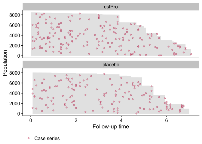
We model the hazard as a function of time, treatment arm and their interaction:
eprchd <- transform(eprchd,
                    treatment = factor(treatment, levels = c("placebo","estPro")))

fit <- fitSmoothHazard(status ~ treatment*ns(time, df = 3),
                       data = eprchd,
                       time = "time")
summary(fit)
#> Fitting smooth hazards with case-base sampling
#>
#> Sample size: 16608
#> Number of events: 324
#> Number of base moments: 32400
#> ----
#>
#> Call:
#> fitSmoothHazard(formula = status ~ treatment * ns(time, df = 3),
#>     data = eprchd, time = "time")
#>
#> Coefficients:
#>                                   Estimate Std. Error z value Pr(>|z|)
#> (Intercept)                       -5.86338    0.29756 -19.705  < 2e-16 ***
#> treatmentestPro                    0.65749    0.37542   1.751   0.0799 .
#> ns(time, df = 3)1                 -0.41771    0.36175  -1.155   0.2482
#> ns(time, df = 3)2                  0.80356    0.72806   1.104   0.2697
#> ns(time, df = 3)3                  1.37487    0.34356   4.002 6.29e-05 ***
#> treatmentestPro:ns(time, df = 3)1  0.06151    0.48825   0.126   0.8997
#> treatmentestPro:ns(time, df = 3)2 -1.40446    0.93844  -1.497   0.1345
#> treatmentestPro:ns(time, df = 3)3 -1.10495    0.48794  -2.265   0.0235 *
#> ---
#> Signif. codes:  0 '***' 0.001 '**' 0.01 '*' 0.05 '.' 0.1 ' ' 1
#>
#> (Dispersion parameter for binomial family taken to be 1)
#>
#>     Null deviance: 3635.4  on 32723  degrees of freedom
#> Residual deviance: 3614.1  on 32716  degrees of freedom
#> AIC: 3630.1
#>
#> Number of Fisher Scoring iterations: 7
Since the output object from fitSmoothHazard inherits
from the glm class, we see a familiar result when using the
function summary.
The treatment effect on the hazard is somewhat difficult to interpret because of its interaction with the spline term on time. In these situations, it is often more instructive to visualize the relationship. For example, we can easily plot the hazard function for each treatment arm:
plot(fit, hazard.params = list(xvar = "time", by = "treatment"))
#> Conditions used in construction of plot
#> treatment: placebo / estPro
#> offset: 0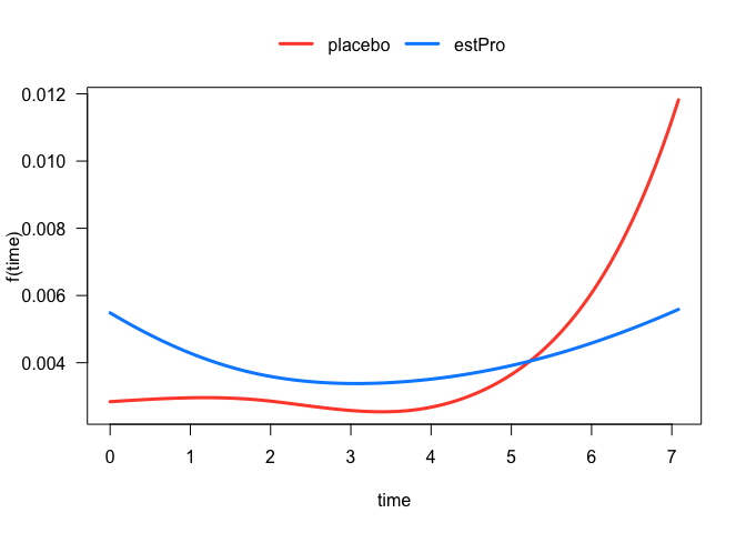
We can also plot the time-dependent hazard ratio and 95% confidence band:
newtime <- quantile(eprchd$time,
                    probs = seq(0.01, 0.99, 0.01))

# reference category
newdata <- data.frame(treatment = factor("placebo",
                                         levels = c("placebo", "estPro")),
                      time = newtime)

plot(fit,
     type = "hr",
     newdata = newdata,
     var = "treatment",
     increment = 1,
     xvar = "time",
     ci = T,
     rug = T)
We can also calculate and plot the cumulative incidence function:
smooth_risk <- absoluteRisk(object = fit,
                            newdata = data.frame(treatment = c("placebo", "estPro")))

plot(smooth_risk, id.names = c("placebo", "estPro"))
The casebase package uses the following hierarchy of
classes for the output of fitSmoothHazard:
casebase:
  singleEventCB:
    - glm
    - gam
    - cv.glmnet
  CompRisk:
    - vglm
The class singleEventCB is an S3 class, and
we also keep track of the classes appearing below. The class
CompRisk is an S4 class that inherits from
vglm.
This package is makes use of several existing packages including:
VGAM for
fitting multinomial logistic regression modelssurvival
for survival modelsggplot2
for plotting the population time plotsdata.table
for efficient handling of large datasetsOther packages with similar objectives but different parametric forms:
citation('casebase')
#> To cite casebase in publications use:
#>
#>   Bhatnagar S, Turgeon M, Islam J, Saarela O, Hanley J (2022).
#>   "casebase: An Alternative Framework for Survival Analysis and
#>   Comparison of Event Rates." _The R Journal_, *14*(3).
#>
#>   Hanley, James A., and Olli S. Miettinen. Fitting smooth-in-time
#>   prognostic risk functions via logistic regression. International
#>   Journal of Biostatistics 5.1 (2009): 1125-1125.
#>
#>   Saarela, Olli. A case-base sampling method for estimating recurrent
#>   event intensities. Lifetime data analysis 22.4 (2016): 589-605.
#>
#> If competing risks analyis is used, please also cite
#>
#>   Saarela, Olli, and Elja Arjas. Non-parametric Bayesian Hazard
#>   Regression for Chronic Disease Risk Assessment. Scandinavian Journal
#>   of Statistics 42.2 (2015): 609-626.
#>
#> To see these entries in BibTeX format, use 'print(<citation>,
#> bibtex=TRUE)', 'toBibtex(.)', or set
#> 'options(citation.bibtex.max=999)'.You can see the most recent changes to the package in the NEWS file
Please note that this project is released with a Contributor Code of Conduct. By participating in this project you agree to abide by its terms.