![]()
![]()
CIFTI files contain brain imaging data in “grayordinates,” which
represent the gray matter as cortical surface vertices (left and right)
and subcortical voxels (cerebellum, basal ganglia, and other deep gray
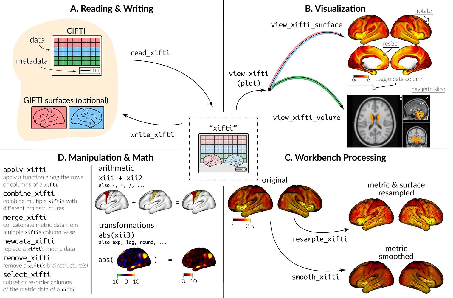
matter). ciftiTools provides a unified environment for
reading, writing, visualizing and manipulating CIFTI-format data. It
supports the “dscalar,” “dlabel,” and “dtseries” intents. Grayordinate
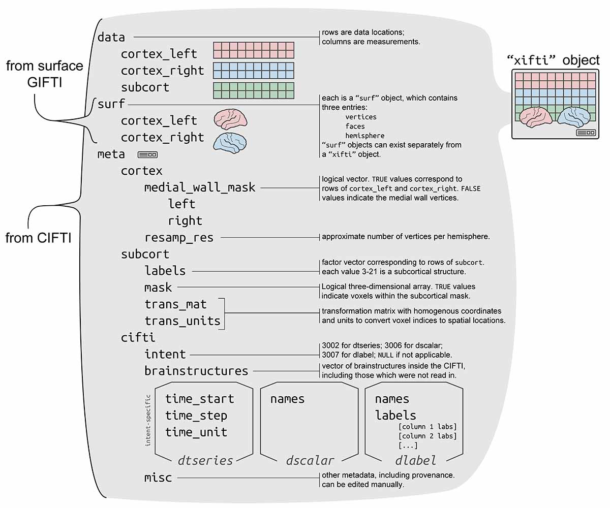
data is read in as a "xifti" object, which is structured
for convenient access to the data and metadata, and includes support for
surface geometry files to enable spatially-dependent functionality such
as static or interactive visualizations and smoothing.
If you use ciftiTools, please cite our paper:
Pham, D. D., Muschelli, J., & Mejia, A. F. (2022). ciftiTools: A package for reading, writing, visualizing, and manipulating CIFTI files in R. NeuroImage, 250, 118877.
You can also obtain citation information from within R like so:
citation("ciftiTools")You can install ciftiTools from CRAN with:
install.packages("ciftiTools")Additionally, most of the ciftiTools functions require
the Connectome Workbench, which can be installed from the HCP
website.
# Load the package and point to the Connectome Workbench --------
library(ciftiTools)
ciftiTools.setOption("wb_path", "path/to/workbench")

# Read and visualize a CIFTI file -------------------------------
cifti_fname <- ciftiTools::ciftiTools.files()$cifti["dtseries"]
surfL_fname <- ciftiTools.files()$surf["left"]
surfR_fname <- ciftiTools.files()$surf["right"]

xii <- read_cifti(
  cifti_fname,
  surfL_fname=surfL_fname, surfR_fname=surfR_fname,
  resamp_res=4000
)

view_xifti_surface(xii) # or plot(xii)
# view_xifti_volume(xii) if subcortex is present

# Access CIFTI data ---------------------------------------------
cortexL <- xii$data$cortex_left
cortexL_mwall <- xii$meta$medial_wall_mask$left
cortexR <- xii$data$cortex_right
cortexR_mwall <- xii$meta$medial_wall_mask$right
# subcortVol <- xii$data$subcort
# subcortLabs <- xii$meta$subcort$labels
# subcortMask <- xii$meta$subcort$mask
surfL <- xii$surf$cortex_left
surfR <- xii$surf$cortex_right

# Create a `"xifti"` from data ----------------------------------
xii2 <- as.xifti(
  cortexL=cortexL, cortexL_mwall=cortexL_mwall,
  cortexR=cortexR, cortexR_mwall=cortexR_mwall,
  #subcortVol=subcortVol, subcortLabs=subcortLabs,
  #subcortMask=subcortMask,
  surfL=surfL, surfR=surfR
)

# Write a CIFTI file --------------------------------------------
write_cifti(xii2, "my_cifti.dtseries.nii")See this link to view the tutorial vignette.
Basics: reading, plotting, writing
ciftiTools.setOption: Necessary to point to the
Connectome Workbench each time ciftiTools is loaded.read_cifti: Read in a CIFTI file as a
"xifti" object.view_xifti Plot the cortex and/or subcortex. Has many
options for controlling the visualization.write_cifti: Write a "xifti" object to a
CIFTI file.Manipulating CIFTI files
resample_cifti: Resample to a different
resolution.separate_cifti: Separate a CIFTI file into GIFTI and
NIFTI files.smooth_cifti: Smooth the data along the surface.run_wb_cmd to execute Connectome Workbench
commands from R)Manipulating "xifti" objects
apply_xifti: Similar to base::apply.combine_xifti: Combine "xifti"s with
non-overlapping brain structures.convert_xifti: Convert between dlabel, dscalar, and
dtseries.impute_xifti: Impute data values from neighboring
vertices/voxels.merge_xifti: Concatenate "xifti"s.move_from_mwall: Convert the medial wall mask to a data
value, deleting the mask.move_to_mwall: Mask out a particular data value.newdata_xifti: Replace the data values.resample_xifti: Resample to a different
resolution.scale_xifti: Similar to base::scale.select_xifti: Rearrange the columns to reorder, take a
subset, or repeat them.smooth_xifti: Smooth the data along the surface.transform_xifti: Apply a vectorizable function.Surface geometry
load_surf: Load a surface geometry included in the
package.read_surf: Read in a GIFTI surface geometry file as a
"surf" object.write_surf: Write a "surf" object to a
GIFTI surface geometry file.Parcellations
apply_parc: Apply a function to each parcel
separately.load_parc: Load a parcellation included in the
package.See NAMESPACE for a full list of all exported
functions.
"xifti"?The "xifti" object is a general interface for not only
CIFTI files, but also GIFTI and NIFTI files. For example, we can plot a
surface GIFTI:
gii_surf <- read_surf(ciftiTools.files()$surf["left"])
xii <- as.xifti(surfL=gii_surf)
plot(xii)
We can also convert metric GIFTI files and/or NIFTI files to CIFTI
files (or vice versa) using the "xifti" object as an
intermediary.
The cortex data will have to be projected to the surface. If the data
are in BIDS format, then fMRIprep can be
used to convert the volumetric cortex data to fsaverage
surface space. Note that ciftiTools::remap_cifti can be
used after to convert from fsaverage to fs_LR
surface space, since some CIFTI-related packages assume the data are
registered to fs_LR. fMRIprep is a wrapper
around FreeSurfer
commands; alternatively, commands from FreeSurfer can be used directly.
Relevant commands include mri_vol2surf,
fslregister, mris_preproc, and
mris_convert. The result of mris_convert will
be in GIFTI format, which can be converted into CIFTI format with
ciftiTools::as.cifti.
More options include those from the Connectome Workbench, ciftify, DeepPrep, and Nilearn. We also welcome input from the community about additional ways for converting from volumetric data to CIFTI format.
Use the Connectome Workbench command -cifti-create-dense-from-template.
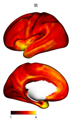
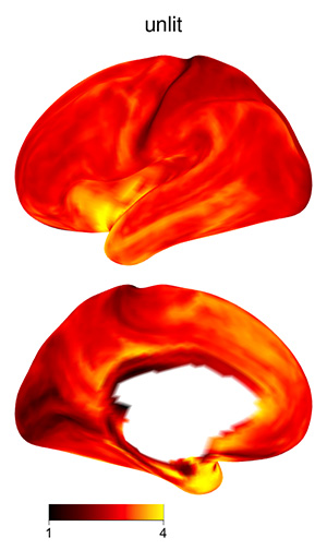
The 3D shading may make certain plots more difficult to interpret, if
the color scale varies from dark to light: darker regions might be in a
shadow, or their values might be lower. To skip shading, use the
argument material=list(lit=FALSE) to
view_xifti_surface.
VoxelIndicesIJK or the MNI coordinates for the
subcortex?For a "xifti" object xii with subcortical
data, the mask of data locations is saved in
xii$meta$subcort$mask. To obtain the array coordinates of
the in-mask locations, use
which(xii$meta$subcort$mask, arr.ind=TRUE) - 1. This matrix
has each subcortical voxel along the rows, and its I, J, and K array
coordinates along the three columns. 1 is subtracted because the
coordinates should begin with 0 rather than 1. It’s equivalent to the
original CIFTI metadata entry VoxelIndicesIJK. To convert
array coordinates to MNI coordinates, multiply by the transformation
matrix xii$meta$subcort$trans_mat:
VoxIJK <- which(xii$meta$subcort$mask, arr.ind=TRUE) - 1
VoxIJK <- cbind(VoxIJK, 1) # for 4th col of transform mat (translation)
VoxXYZ <- t(xii$meta$subcort$trans_mat[seq(3),] %*% t(VoxIJK)) # MNI coordsThe copy of the Yeo 17 parcellation included in
ciftiTools is correct. An earlier figure for the Yeo 17
parcellation had mistakenly swapped these labels, but this error has
since been corrected. See the “Important note” from this page: https://github.com/ThomasYeoLab/CBIG/blob/master/stable_projects/brain_parcellation/Schaefer2018_LocalGlobal/README.md#version-12-schaefer2018_roisparcels_717networks_order
oro.nifti,
RNiftigifticifti
can read in any CIFTI file, whereas ciftiTools provides a
user-friendly interface for CIFTI files with the dscalar, dlabel, and
dtseries intents only.fsbrainxml2rglOn Mac OS Tahoe, Open GL windows will not work due to a problem with
rgl and XQuartz (https://github.com/dmurdoch/rgl/issues/488#issuecomment-3506547361).
To render the cortical surface with plot or
view_xifti_surface, you will need to choose to use the
htmlwidget instead of the Open GL window. Set widget=TRUE
for interactive viewing, and set fname="*.html" to write
files. The ciftiTools development team is currently
exploring workarounds for this issue.
The following data are included in the package for convenience:
Example CIFTI files provided by NITRC.
Cortical surfaces provided by the HCP, according to the Data Use Terms:
Data were provided [in part] by the Human Connectome Project, WU-Minn Consortium (Principal Investigators: David Van Essen and Kamil Ugurbil; 1U54MH091657) funded by the 16 NIH Institutes and Centers that support the NIH Blueprint for Neuroscience Research; and by the McDonnell Center for Systems Neuroscience at Washington University.
Several parcellations provided by Thomas Yeo’s Computational Brain Imaging Group (CBIG):