![]()
Created by Dean Attali
This package provides an interface to explore, analyze, and visualize droplet digital PCR (ddPCR) data in R. It also includes an interactive web application with a visual user interface to facilitate analysis for anyone who is not comfortable with using R. The app is available online or it can be run locally.
This document explains the purpose of this package and includes a tutorial on how to use it. It should take about 20 minutes to go through the entire document. A peer-reviewed publication describing this tool is available in F1000Research.
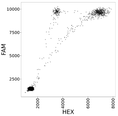
Droplet Digital PCR (ddPCR) is a technology provided by Bio-Rad for performing digital PCR. The basic workflow of ddPCR involves three main steps: partitioning sample DNA into 20,000 droplets, PCR amplification of the nucleic acid in each droplet, and finally passing the droplets through a reader that detects fluorescence in two different wavelengths (generally set to detect FAM and HEX dyes). As a result, the data obtained from a ddPCR experiment can be visualized as a 2D scatterplot (one dimension is FAM intensity and the other dimension is HEX intensity) with 20,000 points (each droplet represents a point). The following figure is an example of a scatterplot from ddPCR data.
This package is designed to analyze two-channel ddPCR experiments (experiments utilizing both fluorescence channels). Single-channel experiments (where only one fluorescence channel is used) cannot use this tool.
A two-channel assay typically uses one FAM dye and one HEX dye, and consequently the droplets will be grouped into one of four clusters: double-positive (droplets that contain both target sequences and emit both HEX and FAM fluorescence), FAM-positive, HEX-positive, and double-negative (empty droplets without any amplifiable template that do not emit fluorescence in either channel). When plotting the droplets, each quadrant of the plot corresponds to a cluster; for example, the droplets in the lower-left quadrant are the double-negative droplets.
After running a ddPCR experiment, a key step in the analysis is gating the droplets to determine how many droplets belong to each cluster. Bio-Rad provides an analysis software called QuantaSoft which can be used to perform gating. QuantaSoft can either do the gating automatically or allow the user to set the gates manually. Most ddPCR users currently gate their data manually because QuantaSoft’s automatic gating often does a poor job and there are no other tools available for gating ddPCR data.
The ddpcr package allows you to import your ddPCR data,
perform some basic analysis, explore the data, and create customizable
figures of the data.
The main features include:
While this tool was originally developed to automatically gate data for a particular ddPCR assay (Quantitative Detection and Resolution of BRAF V600 Status in Colorectal Cancer Using Droplet Digital PCR and a Novel Wild-Type Negative Assay by Roza Bidshahri, Dean Attali, et al.), any ddPCR experiment using an assay with similar characteristics can also use this tool to automatically gate the droplets. In order to benefit from the full automatic analysis, your ddPCR experiment needs to have these characteristics:
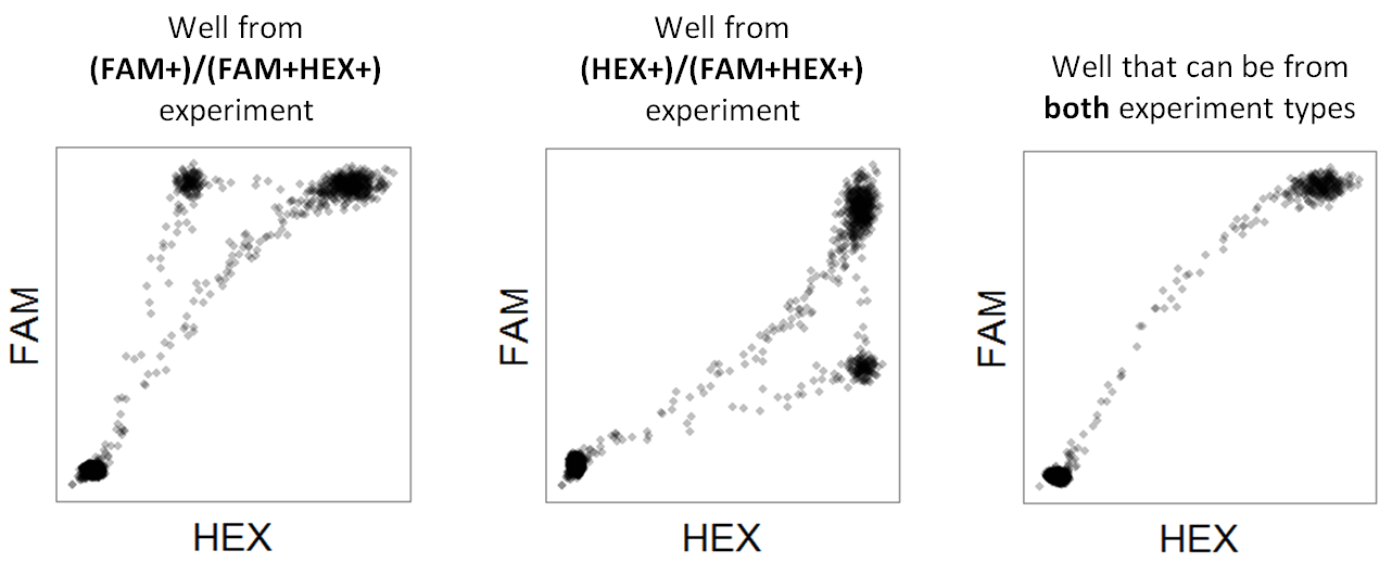
In other words, the built-in automatic gating will work when there are three expected clusters of droplets: (1) double-negative, (2) double-positive, and (3) either FAM+ or HEX+. These types of experiments will be referred to as (FAM+)/(FAM+HEX+) or (HEX+)/(FAM+HEX+). Both of these experiment types fall under the name of PNPP experiments; PNPP is short for PositiveNegative/PositivePositive, which is a reflection of the droplet clusters. Here is what a typical well from a PNPP experiment looks like:
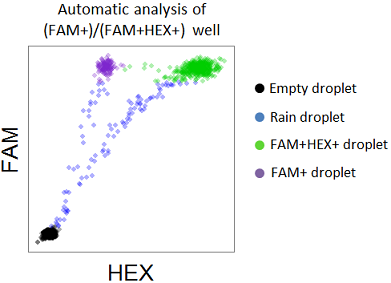
If your experiment matches the criteria for a PNPP experiment (either a (FAM+)/(FAM+HEX+) or a (HEX+)/(FAM+HEX+) experiment), then each droplet will be classified either as a rain droplet or as one of the three expected droplet clusters (FAM+, FAM+HEX+, or double-negative). Rain droplets are droplets that emit considerably more fluorescence than empty droplets, but do not emit enough fluorescence to be assigned into one of the main clusters. Here is the result of analyzing a single well from a (FAM+)/(FAM+HEX+) experiment:
If your ddPCR experiment is not a PNPP type, you can
still use this tool for the rest of the analysis, exploration, and
plotting, but it will not benefit from the automatic gating. However,
ddpcr is built to be easily extensible, which means that
you can add your own experiment type. Custom experiment types need to
define their own method for gating the droplets in a well, and then they
can be used in the same way as the built-in experiment types.
Note: throughout this document, FAM will be synonymous to Y axis and HEX will be synonymous to X axis, as a reflection of the fact that conventionally when visualizing the data the FAM intensity is plotted on the Y axis and the HEX intensity is on the X axis.
If you’re not comfortable using R and would like to use a visual tool that requires no programming, you can use the tool online. You should still skim through the rest of this document (you can ignore the actual code/commands) as it will explain some important concepts.
Enough talking, let’s get our hands dirty.
First, install ddpcr
install.packages("ddpcr")Even if you do know R, using the interactive application can be
easier and more convenient than running R commands. If you want to use
the visual tool, simply run ddpcr::launch() and it will run
the same application that’s hosted online on your own machine.
Here are two basic examples of how to use ddpcr to
analyze and plot your ddPCR data. One example shows an analysis where
the gating thresholds are manually set, and the other example uses the
automated analysis. Explanation will follow, these are just here as a
teaser.
Note how
ddpcris designed to play nicely with the magrittr pipe%>%for easier pipeline workflows.
library(ddpcr)
dir <- sample_data_dir()
# example 1: manually set thresholds
plate1 <-
new_plate(dir, type = plate_types$custom_thresholds) %>%
subset("A01,A05") %>%
set_thresholds(c(5000, 7500)) %>%
analyze()
#> Warning: package 'bindrcpp' was built under R version 3.4.4
plot(plate1, show_grid_labels = TRUE, alpha_drops = 0.3,
title = "Manually set gating thresholds\nworks with any data")
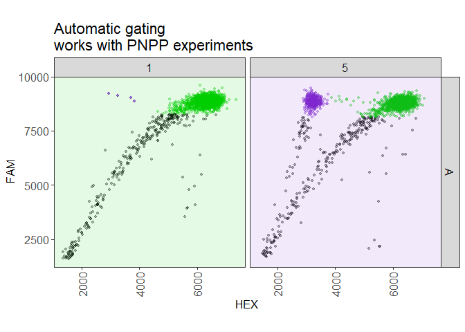
# example 2: automatic gating
new_plate(dir, type = plate_types$fam_positive_pnpp) %>%
subset("A01:A05") %>%
analyze() %>%
plot(show_mutant_freq = FALSE, show_grid_labels = TRUE, alpha_drops = 0.3,
title = "Automatic gating\nworks with PNPP experiments")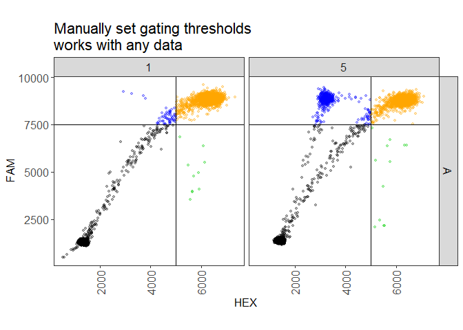
This section will go into details of how to use ddpcr to
analyze ddPCR data.
The first step is to get the ddPCR data into R. ddpcr
uses the data files that are exported by QuantaSoft as its input. If you
loaded an experiment named 2015-05-20_mouse with 50 wells
to QuantaSoft, then QuantaSoft can export the following files:
*_Amplitude.csv. For example, the
droplets in well A01 will be saved in
2015-05-20_mouse_A01_Amplitude.csv (click on the
Export Amplitude and Cluster Data button in the
Setup tab).2015-05-20_mouse.csv
will be generated with some information about the plate, including the
name of the sample in each well (click on the Export
CSV button in the Analyze tab).The well files are the only required input to ddpcr, and
since ddPCR plates contain 96 wells, you can upload anywhere from 1 to
96 well files. The results file is not mandatory, but if you don’t
provide it then the wells will not have sample names attached to
them.
ddpcr contains a sample dataset called
small that has 5 wells. We use the new_plate()
function to initialize a new ddPCR plate object. If given a directory,
it will automatically find all the valid well files in the directory and
attempt to find a matching results file.
library(ddpcr)
dir <- sample_data_dir()
plate <- new_plate(dir)

#> Reading data files into plate... DONE (0 seconds)
#> Initializing plate of type `ddpcr_plate`... DONE (0 seconds)
You will see some messages appear - every time ddpcr
runs an analysis step (initializing the plate is part of the analysis),
it will output a message describing what it’s doing. You can turn off
messages by disabling the verbose option with the command
options(ddpcr.verbose = FALSE).
We can explore the data we loaded even before doing any analysis. The first and easiest thing to do is to plot the raw data.
plot(plate)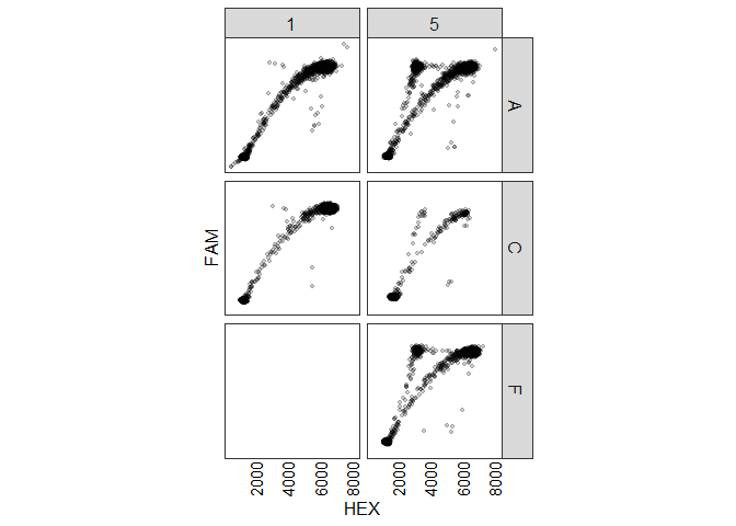
Another way to get a quick overview of the data is by simply printing the plate object.
plate

#>                     ddpcr plate
#>                    -------------
#>             Dataset name : small
#>             Data summary : 5 wells; 72,727 drops
#>               Plate type : ddpcr_plate
#> Completed analysis steps : INITIALIZE
#> Remaining analysis steps : REMOVE_FAILURES, REMOVE_OUTLIERS, REMOVE_EMPTY
Among other things, this tells us how many wells and total droplets we have in the data, and what steps of the analysis are remaining. All the information that gets shown when you print a ddpcr plate object is also available through other functions that are dedicated to show one piece of information. For example
plate %>% name()  # equivalent to `name(plate)`

#> [1] "small"

plate %>% type()  # equivalent to `type(plate)`

#> [1] "ddpcr_plate"
Since we didn’t specify an experiment type, this plate object has the
default type of ddpcr_plate.
We can see what wells are in our data with
wells_used()
plate %>% wells_used()

#> [1] "A01" "A05" "C01" "C05" "F05"
There are 5 wells because the sample data folder has 5 well files.
We can see all the droplets data with plate_data()
plate %>% plate_data()

#> # A tibble: 72,727 x 4
#>    well    HEX   FAM cluster
#>    <chr> <int> <int>   <int>
#>  1 A01     577   494       1
#>  2 A01     515   495       1
#>  3 A01     690   645       1
#>  4 A01     929   860       1
#>  5 A01     844   868       1
#>  6 A01     942   907       1
#>  7 A01     985   923       1
#>  8 A01    1058   966       1
#>  9 A01    1058   979       1
#> 10 A01    1095  1002       1
#> # ... with 72,717 more rows
Technical note: This shows us the fluorescence amplitudes of each droplet, along with the current cluster assignment of each droplet. Right now all droplets are assigned to cluster 1 which corresponds to undefined since no analysis has taken place yet. You can see all the clusters that a droplet can belong to with the
clusters()functionplate %>% clusters() #> [1] "UNDEFINED" "FAILED" "OUTLIER" "EMPTY"This tells us that any droplet in a
ddpcr_plate-type experiment can be classified into those clusters. Any droplet is initially UNDEFINED, droplets in failed wells are marked as FAILED, and the other two names are self-explanatory.
We can see the results of the plate so far with
plate_meta()
plate %>% plate_meta(only_used = TRUE)

#>   well sample row col used    target_ch1     target_ch2 drops
#> 1  A01   Dean   A   1 TRUE Consensus_FAM WTspecific_HEX 15820
#> 2  A05   Dave   A   5 TRUE Consensus_FAM WTspecific_HEX 13165
#> 3  C01   Mike   C   1 TRUE Consensus_FAM WTspecific_HEX 14256
#> 4  C05  Emily   C   5 TRUE Consensus_FAM WTspecific_HEX 14109
#> 5  F05   Mary   F   5 TRUE Consensus_FAM WTspecific_HEX 15377
The only_used parameter is used so that we’ll only get
data about the 5 existing wells and ignore the other 91 unused wells on
the plate. Notice that meta (short for metadata) is
used instead of results. This is because the meta/results table
contains information for each well such as its name, number of drops,
number of empty drops, concentration, and many other calculated
values.
If you aren’t interested in all the wells, you can use the
subset() function to retain only certain wells.
Alternatively, you can use the data_files argument of the
new_plate() function to only load certain well files
instead of a full directory.
The subset() function accepts either a list of sample
names, a list of wells, or a special range notation. The range
notation is a convenient way to select many wells: use a colon
(:) to specify a range of wells and a comma
(,) to add another well or range. A range of wells is
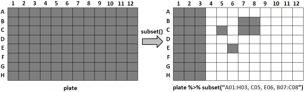
defined as all wells in the rectangular area between the two endpoints.
For example, B05:C06 corresponds to the four wells
B05, B06, C05, C06. The following diagram shows the result
of subsetting with a range notation of
A01:H03, C05, E06, B07:C08 on a plate that initially
contains all 96 wells.
Back to our data: we have 5 wells, let’s keep 4 of them
plate <- plate %>% subset("A01:C05")
# could have also used subset("A01, A05, C01, C05")
plate %>% wells_used()

#> [1] "A01" "A05" "C01" "C05"An analysis of a ddPCR plate consists of running the plate through a sequence of steps. You can see the steps of an experiment by printing it.
plate

#>                     ddpcr plate
#>                    -------------
#>             Dataset name : small
#>             Data summary : 4 wells; 57,350 drops
#>               Plate type : ddpcr_plate
#> Completed analysis steps : INITIALIZE
#> Remaining analysis steps : REMOVE_FAILURES, REMOVE_OUTLIERS, REMOVE_EMPTY
The last two lines show which steps have been completed and which
steps remain. These steps are the default steps that any ddpcr plate
will go through by default if no type is specified. At this point all we
did was load the data, so the initialization step was done and there are
3 remaining steps. You can run all remaining steps with
analyze(), or run through the steps one by one using
next_step().
plate <- plate %>% analyze()

#> Identifying failed wells... DONE (0 seconds)
#> Identifying outlier droplets... DONE (0 seconds)
#> Identifying empty droplets... DONE (1 seconds)
#> Analysis complete

# equivalent to `plate %>% next_step(3)`
# also equivalent to `plate %>% next_step() %>% next_step() %>% next_step()`
As each step of the analysis is performed, a message describing the current step is printed to the screen. Since we only have 4 wells, it should be very fast, but when you have a full 96-well plate, the analysis could take several minutes. Sometimes it can be useful to run each step individually rather than all of them together if you want to inspect the data after each step.
We can explore the plate again, now that it has been analyzed.
plate

#>         ddpcr plate
#>        -------------
#> Dataset name : small
#> Data summary : 4 wells; 57,350 drops
#>   Plate type : ddpcr_plate
#>       Status : Analysis completed
We now get a message that says the analysis is complete (earlier it said which steps were remaining). We can also look at the droplets data
plate %>% plate_data()

#> # A tibble: 57,350 x 4
#>    well    HEX   FAM cluster
#>    <chr> <int> <int>   <int>
#>  1 A01     577   494       4
#>  2 A01     515   495       4
#>  3 A01     690   645       4
#>  4 A01     929   860       4
#>  5 A01     844   868       4
#>  6 A01     942   907       4
#>  7 A01     985   923       4
#>  8 A01    1058   966       4
#>  9 A01    1058   979       4
#> 10 A01    1095  1002       4
#> # ... with 57,340 more rows
This isn’t very informative since it shows the cluster assignment for each droplet, which is not easy for a human to digest. Instead, this information can be visualized by plotting the plate (coming up). We can also look at the plate results
plate %>% plate_meta(only_used = TRUE)

#>   well sample row col used    target_ch1     target_ch2 drops success
#> 1  A01   Dean   A   1 TRUE Consensus_FAM WTspecific_HEX 15820    TRUE
#> 2  A05   Dave   A   5 TRUE Consensus_FAM WTspecific_HEX 13165    TRUE
#> 3  C01   Mike   C   1 TRUE Consensus_FAM WTspecific_HEX 14256    TRUE
#> 4  C05  Emily   C   5 TRUE Consensus_FAM WTspecific_HEX 14109   FALSE
#>   drops_outlier drops_empty drops_non_empty drops_empty_fraction
#> 1             2       13690            2130                0.865
#> 2             1       11283            1882                0.857
#> 3             0       12879            1377                0.903
#> 4             0          NA              NA                   NA
#>   concentration
#> 1           170
#> 2           181
#> 3           120
#> 4            NA
Now there’s a bit more information in the results table. The
success column indicates whether or not the ddPCR run was
successful in that particular well; notice how well C05 was
deemed a failure, and thus is not included the any subsequent analysis
steps.
You can use the well_info() function to get the value of
a specific variable of a specific well from the results. For example, we
can query the plate object to see how many empty droplets are in well
A05.
well_info(plate, "A05", "drops_empty")

#> [1] 11283The easiest way to visualize a ddPCR plate is using the
plot() function.
plate %>% plot()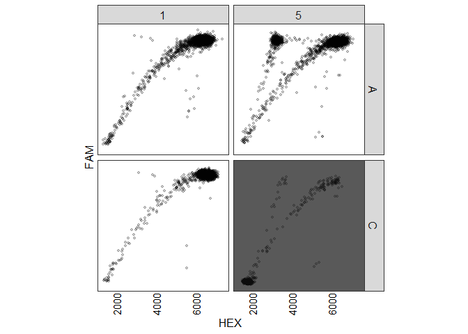
Notice well C05 is grayed out, which means that it is a
failed well. By default, failed wells have a grey background, and empty
and outlier droplets are excluded from the plot.
You don’t have to analyze a plate object before you can plot it - a ddPCR plate can be plotted at any time to show the data in it. If you plot a plate before analyzing it, it’ll show the raw data.
There are many plot parameters to allow you to create extremely
customizable plots. Among the many parameters, there are three special
categories of parameters that affect the visibility of droplets:
show_drops_* is used to show/hide certain droplets,
col_drops_* is used to set the colour of droplets, and
alpha_drops_* is used to set the transparency of droplets
(0 = transparent, 1 = opaque). The * can be replaced by the
name of any droplet cluster (the available clusters can be obtained with
clusters(plate) as mentioned earlier). For example, to show
the outlier droplets in blue, add the parameters
show_drops_outlier = TRUE, col_drops_outlier = "blue".
The following two plots show examples of how to use some plot parameters.
plate %>% plot(wells = "A01,A05", show_full_plate = TRUE,
show_drops_empty = TRUE, col_drops_empty = "red",
title = "Show full plate")
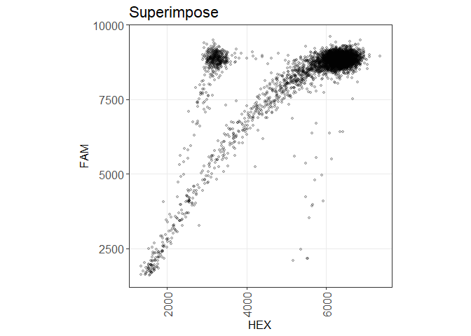
plate %>% plot(wells = "A01,A05", superimpose = TRUE,
show_grid = TRUE, show_grid_labels = TRUE, title = "Superimpose")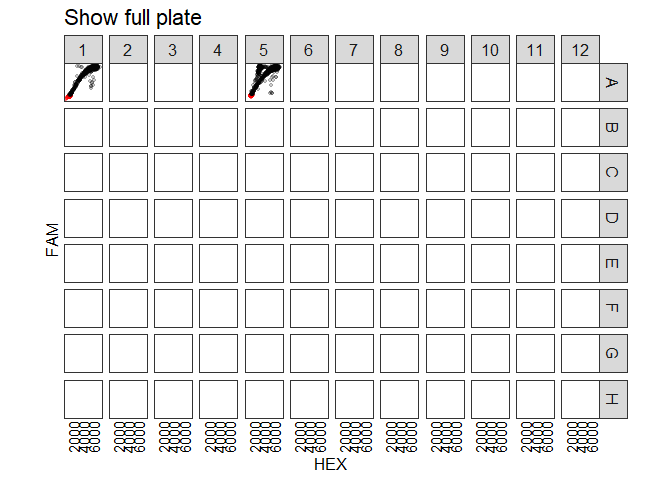
To see all the available plot parameters, run
?plot.ddpcr_plate.
As was shown previously, you can use the plate_meta()
function to retrieve a table with the results. If you want to save that
table, you can use R’s built-in write.csv() or
write.table() functions.
You can also save a ddPCR plate object using
plate_save(). This will create a single .rds
file that contains an exact copy of the plate’s current state, including
all the data, attributes, and analysis progress of the plate. The
resulting file can be loaded to restore the ddPCR object at a later time
with plate_load().
plate %>% save_plate("myplate")
from_file <- load_plate("myplate")
identical(plate, from_file)

#> [1] TRUE

unlink("myplate.rds")So far we only used the default plate type in this analysis, but droplet gating does not take place with the default type. While you can define your own plate types (more on that later), there are three built-in plate types you can use:
plate_types$custom_thresholds - when
you want to gate your droplets into four quadrants according to HEX and
FAM values that you setplate_types$fam_positive_pnpp - when
you have a FAM-positive PNPP plate (FAM+)/(FAM+HEX+)plate_types$hex_positive_pnpp - when
you have a HEX-positive PNPP plate (HEX+)/(FAM+HEX+)The next two sections explain how to use these experiment types.
If you want to perform a simple 4-quadrant gating like the one
available in QuantaSoft, you need to set the type of the plate object to
plate_types$custom_thresholds. This can either be done when
initializing a new plate or by resetting an existing plate object.
# two ways to create the desired plate
plate_manual <- reset(plate, type = plate_types$custom_thresholds)
plate_manual2 <- new_plate(dir, type = plate_types$custom_thresholds) %>%
  subset("A01:C05")

# make sure the two methods above are identical
identical(plate_manual, plate_manual2)

#> [1] TRUE

plate_manual

#>                     ddpcr plate
#>                    -------------
#>             Dataset name : small
#>             Data summary : 4 wells; 57,350 drops
#>               Plate type : custom_thresholds, ddpcr_plate
#> Completed analysis steps : INITIALIZE
#> Remaining analysis steps : REMOVE_OUTLIERS, CLASSIFY
It’s usually a good idea to take a look at the raw data to decide where the draw the thresholds
plot(plate_manual, show_grid_labels = TRUE)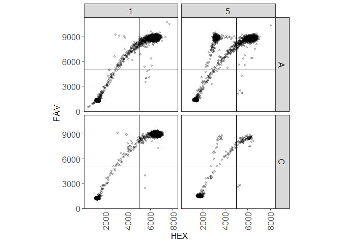
If you noticed, there’s a droplet in well A05 that has a much larger fluorescence value and is probably an outlier, which is the reason the scale is a bit too large. After analyzing the plate, it will be identified as an outlier and hidden automatically. Before running the analysis, we should set where the thresholds will be. By default, the thresholds are at (5000, 5000), which is very arbitrary. It looks like the x coordinate is fine, but the y border should move up to approximately 8000. Then run the analysis.
# what are the current thresholds?
thresholds(plate_manual)

#> [1] "(5000, 5000)"

# set the thresholds to (5000,8000)
thresholds(plate_manual) <- c(5000, 8000)
plate_manual <- analyze(plate_manual)

#> Identifying outlier droplets... DONE (0 seconds)
#> Classifying droplets... DONE (0 seconds)
#> Analysis complete
Now the plate is ready and we can plot it or look at its results
plate_meta(plate_manual, only_used = TRUE)

#>   well sample row col used    target_ch1     target_ch2 drops
#> 1  A01   Dean   A   1 TRUE Consensus_FAM WTspecific_HEX 15820
#> 2  A05   Dave   A   5 TRUE Consensus_FAM WTspecific_HEX 13165
#> 3  C01   Mike   C   1 TRUE Consensus_FAM WTspecific_HEX 14256
#> 4  C05  Emily   C   5 TRUE Consensus_FAM WTspecific_HEX 14109
#>   drops_outlier drops_empty drops_x_positive drops_y_positive
#> 1             2       13909               20               20
#> 2             1       11512               34              390
#> 3             0       12967                8                7
#> 4             0       14011               15               11
#>   drops_both_positive
#> 1                1869
#> 2                1228
#> 3                1274
#> 4                  72

plot(plate_manual)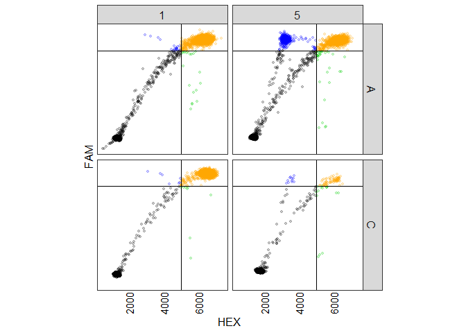
By default, the droplets in each quadrant are a different colour. If
you want to change the colour of some droplets, we can use the
col_drops_* parameter as before. Since now we’re working
with a different plate type, the names of the droplet clusters can be
different, so we need to first know what they are
clusters(plate_manual)

#> [1] "UNDEFINED"     "OUTLIER"       "EMPTY"         "X_POSITIVE"
#> [5] "Y_POSITIVE"    "BOTH_POSITIVE"
Now if we want to change the colour of the double-positive droplets
to red, we just add a parameter
col_drops_both_positive = "red".
To see all the available plot parameters for this plate type, run
?plot.custom_thresholds. In addition, any plot parameter that is available for default plates can also be used here (all parameters listed under?plot.ddpcr_plate).
If you have a PNPP experiment ((FAM+)/(FAM+HEX+) or
(HEX+)/(FAM+HEX+)), then ddpcr can perform a fully
automatic analysis on the plate. The sample dataset used in this running
example is from a (FAM+)/(FAM+HEX+) experiment, so we can take
advantage of the automatic gating if we set the type to
plate_types$fam_positive_pnpp.
Let’s create a new plate object of the desired type.
plate_pnpp <- new_plate(dir, type = plate_types$fam_positive_pnpp)

#> Reading data files into plate... DONE (0 seconds)
#> Initializing plate of type `fam_positive_pnpp`... DONE (0 seconds)
If the data were (HEX+)/(FAM+HEX+), we would have used
type = plate_types$hex_positive_pnpp instead.
Before running the analysis, it’s a good idea to know what are the possible cluster groupings that a droplet can belong to
clusters(plate_pnpp)

#> [1] "UNDEFINED" "FAILED"    "OUTLIER"   "EMPTY"     "RAIN"      "POSITIVE"
#> [7] "NEGATIVE"
The first 4 clusters we’ve seen before, as they are common to all plate types. Droplets in the HEX+FAM+ cluster are considered POSITIVE, while droplets in the FAM+ cluster are considered NEGATIVE since they are HEX-. Any droplets that are not empty but don’t emit enough fluorescent intensity to be in the POSITIVE or NEGATIVE clusters are considered RAIN.
When using the
plate_types$fam_positive_pnpptype, the positive droplets (FAM+HEX+) are called wildtype, and the negative droplets (FAM+HEX-) are called mutant. Why? This package was originally designed to analyze a specific assay where the FAM+HEX+ cluster represented droplets with a wildtype gene inside, while the FAM+HEX- cluster corresponded to droplets with a mutant gene. Talking about positive vs negative drops or positive vs negative wells sounds a bit weird, so it was decided to stick with mutant vs wildtype. Just remember: wildtype = double-positive droplets, mutant = singly-positive droplets.
Now we can analyze the plate
plate_pnpp <- analyze(plate_pnpp)

#> Identifying failed wells... DONE (0 seconds)
#> Identifying outlier droplets... DONE (0 seconds)
#> Identifying empty droplets... DONE (0 seconds)
#> Classifying droplets... DONE (0 seconds)
#> Reclassifying droplets... skipped (not enough wells with significant mutant clusters)
#> Analysis complete
One of the key goals in running the analysis is to determine the number of POSITIVE (wildtype) and NEGATIVE (mutant) droplets in each well, and similarly the mutant frequency (if a well has 95 wildtype droplets and 5 mutant droplets, then the mutant frequency in the well is 5%).
You can see from the output that the two last steps are classifying and reclassifying the droplets, and that the reclassification didn’t take place. The classification step identifies all the non-empty droplets as either rain, mutant, or wildtype by analyzing each well individually. Wells with a very low mutant frequency (i.e. there are very few mutant droplets) are much harder to gate accurately, which is the reason for the reclassification step. The reclassification step uses information from wells with high a mutant frequency, where the gates are more clearly defined, to adjust the gates in wells with a low mutant frequency. The reclassification step only takes place if there are enough wells with a high mutant frequency.
Take a look at the results
plate_pnpp %>% plate_meta(only_used = TRUE)

#>   well sample row col used    target_ch1     target_ch2 drops success
#> 1  A01   Dean   A   1 TRUE Consensus_FAM WTspecific_HEX 15820    TRUE
#> 2  A05   Dave   A   5 TRUE Consensus_FAM WTspecific_HEX 13165    TRUE
#> 3  C01   Mike   C   1 TRUE Consensus_FAM WTspecific_HEX 14256    TRUE
#> 4  F05   Mary   F   5 TRUE Consensus_FAM WTspecific_HEX 15377    TRUE
#> 5  C05  Emily   C   5 TRUE Consensus_FAM WTspecific_HEX 14109   FALSE
#>   drops_outlier drops_empty drops_non_empty drops_empty_fraction
#> 1             2       13690            2130                0.865
#> 2             1       11283            1882                0.857
#> 3             0       12879            1377                0.903
#> 4             0       14126            1251                0.919
#> 5             0          NA              NA                   NA
#>   concentration mutant_border filled_border significant_mutant_cluster
#> 1           170          4194          8286                      FALSE
#> 2           181          3789          8136                       TRUE
#> 3           120          4356          8445                      FALSE
#> 4            99          3926          8294                       TRUE
#> 5            NA            NA            NA                         NA
#>   mutant_num wildtype_num mutant_freq
#> 1          4         1827       0.218
#> 2        368         1224      23.100
#> 3          3         1248       0.240
#> 4        211          855      19.800
#> 5         NA           NA          NA
Explanation of some of the variables:
Plotting the data is usually the best way to see the results
plate_pnpp %>% plot(text_size_mutant_freq = 8)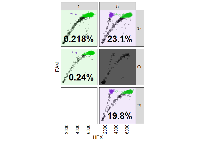
To see all the available plot parameters for this plate type, run
?plot.pnpp_experiment. In addition, any plot parameter that is available for default plates can also be used here (all parameters listed under?plot.ddpcr_plate).
The wildtype droplets are green and the mutant droplets are purple. The well colours themselves reflect the significant_mutant_cluster variable: wells that are mostly wildtype droplets are green, and wells with significant mutant clusters are purple. There are parameters to set all these colours, the transparency levels, and many more options.
Similar to how wells_failed() returns the failed wells,
you can use the wells_mutant() and
wells_wildtype() functions to extract the wells with a
significant mutant cluster and those without.
plate_pnpp %>% wells_mutant()

#> [1] "A05" "F05"

plate_pnpp %>% wells_wildtype()

#> [1] "A01" "C01"Every ddPCR plate object has adjustable parameters associated with
it. There are general parameters that apply to the plate as a whole, and
each analysis step has its own set of parameters that are used for the
algorithm in that step. You can see all the parameters of a plate using
the params() function
plate %>% params() %>% str()

#> List of 4
#>  $ GENERAL        :List of 4
#>   ..$ X_VAR         : chr "HEX"
#>   ..$ Y_VAR         : chr "FAM"
#>   ..$ DROPLET_VOLUME: num 0.00085
#>   ..$ RANDOM_SEED   : num 8
#>  $ REMOVE_FAILURES:List of 3
#>   ..$ TOTAL_DROPS_T      : num 5000
#>   ..$ EMPTY_LAMBDA_LOW_T : num 0.3
#>   ..$ EMPTY_LAMBDA_HIGH_T: num 0.99
#>  $ REMOVE_OUTLIERS:List of 2
#>   ..$ TOP_PERCENT: num 1
#>   ..$ CUTOFF_IQR : num 5
#>  $ REMOVE_EMPTY   :List of 1
#>   ..$ CUTOFF_SD: num 7
You can also view the parameters for a specific step or the value of a parameter. For example, to see the parameters used in the step that identifies failed wells, use
plate %>% params("REMOVE_FAILURES")

#> $TOTAL_DROPS_T
#> [1] 5000
#>
#> $EMPTY_LAMBDA_LOW_T
#> [1] 0.3
#>
#> $EMPTY_LAMBDA_HIGH_T
#> [1] 0.99
You can also view or edit specific parameters. When identifying
failed wells, one of the conditions for a successful run is to have at
least 5,000 droplets in the well (Bio-Rad claims that every well has
20,000 droplets). If you know that your particular experiment had much
fewer droplets than usual and as a result ddpcr thinks that
all the wells are failures, you can change the setting
params(plate, "REMOVE_FAILURES", "TOTAL_DROPS_T")

#> [1] 5000

params(plate, "REMOVE_FAILURES", "TOTAL_DROPS_T") <- 1000
params(plate, "REMOVE_FAILURES", "TOTAL_DROPS_T")

#> [1] 1000
If you look at the full parameters of the plate, you’ll notice that
by default ddpcr assumes that the dyes used are
FAM and HEX. If you are using a different dye and want
the name of that dye appear in the results instead, you can use the
x_var() or y_var() functions.
orig_x <- x_var(plate)
orig_x

#> [1] "HEX"

x_var(plate) <- "VIC"
plate %>% plate_data() %>% names()

#> [1] "well"    "VIC"     "FAM"     "cluster"

x_var(plate) <- orig_x
Note that if you change any parameters, you need to re-run the
analysis. If you try running analyze() after a plate has
already been analyzed, you will simply get a message saying the plate is
already analyzed. To force an already-analyzed plate to re-run the
analysis, you need to use the restart = TRUE parameter.
plate <- analyze(plate)

#> Analysis complete

plate <- analyze(plate, restart = TRUE)

#> Restarting analysis

#> Initializing plate of type `ddpcr_plate`... DONE (0 seconds)
#> Identifying failed wells... DONE (0 seconds)
#> Identifying outlier droplets... DONE (0 seconds)
#> Identifying empty droplets... DONE (1 seconds)
#> Analysis completeIf you want to know how a step is performed, you can see the exact
algorithm (code) used in each step by consulting the
steps() function.
plate_pnpp %>% steps

#> $INITIALIZE
#> [1] "init_plate"
#>
#> $REMOVE_FAILURES
#> [1] "remove_failures"
#>
#> $REMOVE_OUTLIERS
#> [1] "remove_outliers"
#>
#> $REMOVE_EMPTY
#> [1] "remove_empty"
#>
#> $CLASSIFY
#> [1] "classify_droplets"
#>
#> $RECLASSIFY
#> [1] "reclassify_droplets"
This list contains all the steps of analyzing the given plate, with
each item in the list containing both the name of the step and the R
function that performs it. For example, the first step is
INITIALIZE and it uses the function init_plate().
You can see the code for that function by running
ddpcr:::init_plate.
ddpcr:::init_plate

#> function(plate) {
#>   stopifnot(plate %>% inherits("ddpcr_plate"))
#>   step_begin(sprintf("Initializing plate of type `%s`", type(plate)))
#>
#>   plate %<>%
#>     set_default_clusters %>%
#>     set_default_steps %>%
#>     init_data %>%
#>     init_meta
#>
#>   status(plate) <- step(plate, 'INITIALIZE')
#>   plate[['version']] <- as.character(utils::packageVersion("ddpcr"))
#>   plate[['dirty']] <- FALSE
#>   step_end()
#>
#>   plate
#> }
#> <environment: namespace:ddpcr>
For more details about the algorithm, see the Algorithms vignette.
Each ddPCR plate has a plate type which determines what type of
analysis to run on the data. plate_types contains a list of
the built-in plate types that are supported, but you can also create
your own plate type. Create a new plate type if you want to supply your
own logic for any analysis step, or even if you simply want to have a
type that sets different default parameters than the built-in ones.
For more details about how to create new plate types, see the Extending ddpcr by adding new plate types vignette.
The ddpcr package uses some advanced R programming
techniques.
For details on the technical details regarding the code implementation, see the Technical details vignette.