
![]()
![]()
![]()
detectseparation provides pre-fit and post-fit methods for the detection of separation and of infinite maximum likelihood estimates in binomial response generalized linear models.
The key methods are detect_infinite_estimates(),
detect_separation() and
check_infinite_estimates().
You can install the released version of detectseparation from CRAN with:
install.packages("detectseparation")and the development version from GitHub with:
# install.packages("devtools")
devtools::install_github("ikosmidis/detectseparation", ref = "develop")Heinze and Schemper (2002) used a logistic regression model to
analyze data from a study on endometrial cancer (see, Agresti 2015,
sec. 5.7 or ?endometrial for more details on the data set).
Below, we refit the model in Heinze and Schemper (2002) in order to
demonstrate the functionality that detectseparation
provides.
library("detectseparation")
data("endometrial", package = "detectseparation")
endo_glm <- glm(HG ~ NV + PI + EH, family = binomial(), data = endometrial)
theta_mle <- coef(endo_glm)
summary(endo_glm)
#>
#> Call:
#> glm(formula = HG ~ NV + PI + EH, family = binomial(), data = endometrial)
#>
#> Coefficients:
#>               Estimate Std. Error z value Pr(>|z|)
#> (Intercept)    4.30452    1.63730   2.629 0.008563 **
#> NV            18.18556 1715.75089   0.011 0.991543
#> PI            -0.04218    0.04433  -0.952 0.341333
#> EH            -2.90261    0.84555  -3.433 0.000597 ***
#> ---
#> Signif. codes:  0 '***' 0.001 '**' 0.01 '*' 0.05 '.' 0.1 ' ' 1
#>
#> (Dispersion parameter for binomial family taken to be 1)
#>
#>     Null deviance: 104.903  on 78  degrees of freedom
#> Residual deviance:  55.393  on 75  degrees of freedom
#> AIC: 63.393
#>
#> Number of Fisher Scoring iterations: 17
The maximum likelihood (ML) estimate of the parameter for
NV is actually infinite. The reported, apparently finite
value is merely due to false convergence of the iterative estimation
procedure. The same is true for the estimated standard error, and, hence
the value 0.011 for the z-statistic cannot be trusted for
inference on the size of the effect for NV.
detect_separation()detect_separation() is a pre-fit method, in the
sense that it does not need to estimate the model to detect separation
and/or identify infinite estimates. For example,
endo_sep <- glm(HG ~ NV + PI + EH, data = endometrial,
                family = binomial("logit"),
                method = "detect_separation")
endo_sep
#> Implementation: ROI | Solver: lpsolve
#> Separation: TRUE
#> Existence of maximum likelihood estimates
#> (Intercept)          NV          PI          EH
#>           0         Inf           0           0
#> 0: finite value, Inf: infinity, -Inf: -infinity
So, the actual maximum likelihood estimates are
coef(endo_glm) + coef(endo_sep)
#> (Intercept)          NV          PI          EH
#>   4.3045178         Inf  -0.0421834  -2.9026056
and the estimated standard errors are
coef(summary(endo_glm))[, "Std. Error"] + abs(coef(endo_sep))
#> (Intercept)          NV          PI          EH
#>  1.63729861         Inf  0.04433196  0.84555156
We can ask detect_separation() not only to detect
separation, but also, if separation is detected, to solve an additional
linear program to check whether separation is complete or
quasi-complete. We do this by setting
separation_type = TRUE in the glm() call
glm(HG ~ NV + PI + EH, data = endometrial, family = binomial("logit"),
    method = "detect_separation", separation_type = TRUE)
#> Implementation: ROI | Solver: lpsolve
#> Separation: TRUE (quasi-complete)
#> Existence of maximum likelihood estimates
#> (Intercept)          NV          PI          EH
#>           0         Inf           0           0
#> 0: finite value, Inf: infinity, -Inf: -infinity
We can of course, simply, use the update method on the
glm object, if that is available, and change the
method argument with any extra options. For example,
update(endo_glm, method = "detect_separation", separation_type = TRUE)
#> Implementation: ROI | Solver: lpsolve
#> Separation: TRUE (quasi-complete)
#> Existence of maximum likelihood estimates
#> (Intercept)          NV          PI          EH
#>           0         Inf           0           0
#> 0: finite value, Inf: infinity, -Inf: -infinitycheck_infinite_estimates()Lesaffre and Albert (1989, sec. 4) describe a procedure that can hint
on the occurrence of infinite estimates. In particular, the model is
successively refitted, by increasing the maximum number of allowed
iteratively re-weighted least squares iterations at each step. The
estimated asymptotic standard errors from each step are, then, divided
to the corresponding ones from the first fit. If the sequence of ratios
diverges, then the maximum likelihood estimate of the corresponding
parameter is minus or plus infinity. The following code chunk applies
this process to endo_glm.
(inf_check <- check_infinite_estimates(endo_glm))
#>       (Intercept)           NV       PI       EH
#>  [1,]    1.000000 1.000000e+00 1.000000 1.000000
#>  [2,]    1.424352 2.092407e+00 1.466885 1.672979
#>  [3,]    1.590802 8.822303e+00 1.648003 1.863563
#>  [4,]    1.592818 6.494231e+01 1.652508 1.864476
#>  [5,]    1.592855 7.911035e+02 1.652591 1.864492
#>  [6,]    1.592855 1.588973e+04 1.652592 1.864493
#>  [7,]    1.592855 5.298760e+05 1.652592 1.864493
#>  [8,]    1.592855 2.332822e+07 1.652592 1.864493
#>  [9,]    1.592855 2.332822e+07 1.652592 1.864493
#> [10,]    1.592855 2.332822e+07 1.652592 1.864493
#> [11,]    1.592855 2.332822e+07 1.652592 1.864493
#> [12,]    1.592855 2.332822e+07 1.652592 1.864493
#> [13,]    1.592855 2.332822e+07 1.652592 1.864493
#> [14,]    1.592855 2.332822e+07 1.652592 1.864493
#> [15,]    1.592855 2.332822e+07 1.652592 1.864493
#> [16,]    1.592855 2.332822e+07 1.652592 1.864493
#> [17,]    1.592855 2.332822e+07 1.652592 1.864493
#> [18,]    1.592855 2.332822e+07 1.652592 1.864493
#> [19,]    1.592855 2.332822e+07 1.652592 1.864493
#> [20,]    1.592855 2.332822e+07 1.652592 1.864493
#> attr(,"class")
#> [1] "inf_check"
plot(inf_check)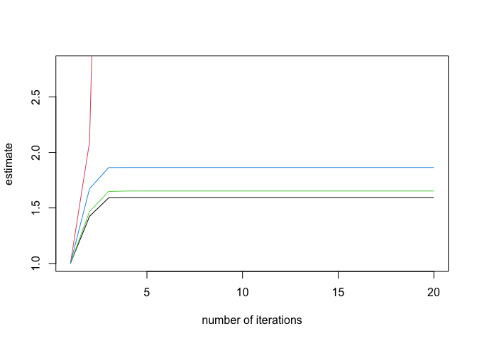
Agresti, A. 2015. Foundations of Linear and Generalized Linear Models. Wiley Series in Probability and Statistics. Wiley.
Heinze, G., and M. Schemper. 2002. “A Solution to the Problem of Separation in Logistic Regression.” Statistics in Medicine 21: 2409–19.
Lesaffre, E., and A. Albert. 1989. “Partial Separation in Logistic Discrimination.” Journal of the Royal Statistical Society. Series B (Methodological) 51 (1): 109–16. https://www.jstor.org/stable/2345845.