

![]()
![]()
![]()
![]()
![]()
Tools to Retrieve Economic Policy Institute Data Library Extracts
The Economic Policy Institute (https://www.epi.org/) provides researchers, media, and the public with easily accessible, up-to-date, and comprehensive historical data on the American labor force. It is compiled from Economic Policy Institute analysis of government data sources. Use it to research wages, inequality, and other economic indicators over time and among demographic groups. Data is usually updated monthly.
The following functions are implemented:
get_annual_wages_and_work_hours: Retreive CPS ASEC
Annual Wages and Work Hoursget_annual_wages_by_wage_group: Annual wages by wage
groupget_black_white_wage_gap: Retreive the percent by which
hourly wages of black workers are less than hourly wages of white
workersget_college_wage_premium: Retreive the percent by which
hourly wages of college graduates exceed those of otherwise equivalent
high school graduatesget_compensation_wages_and_benefits: Compensation,
wages, and benefitsget_employment_to_population_ratio: Retreive the share
of the civilian noninstitutional population that is employedget_gender_wage_gap: Retreive the percent by which
hourly wages of female workers are less than hourly wages of male
workersget_health_insurance_coverage: Retreive Health
Insurance Coverageget_hispanic_white_wage_gap: Retreive the percent by
which hourly wages of Hispanic workers are less than hourly wages of
white workersget_labor_force_participation_rate: Retreive the share
of the civilian noninstitutional population that is in the labor
forceget_long_term_unemployment: Retreive the share of the
labor force that has been unemployed for six months or longerget_median_and_mean_wages: Retreive the hourly wage in
the middle of the wage distributionget_minimum_wage: Minimum wageget_non_high_school_wage_penalty: Retreive the percent
by which hourly wages of workers without a high school diploma (or
equivalent) are less than wages of otherwise equivalent workers who have
graduated from high schoolget_pension_coverage: Retreive Pension Coverageget_poverty_level_wages: Poverty-level wagesget_productivity_and_hourly_compensation: Retreive
Productivity and hourly compensationget_underemployment: Retreive the share of the labor
force that is “underemployed”get_unemployment_by_state: Retreive the share of the
labor force without a job (by state)get_unemployment: Retreive the share of the labor force
without a jobget_union_coverage: Retreive Union Coverageget_wage_decomposition: Retreive Wage
Decompositionget_wages_by_education: Retreive the average hourly
wages of workers disaggregated by the highest level of education
attainedget_wages_by_percentile: Retreive wages at ten distinct
points in the wage distributionnot_dos: Not DoS’ing EPI/Cloudflareinstall.packages("epidata") # NOTE: CRAN version is 0.3.0
# or
install.packages("epidata", repos = c("https://cinc.rud.is", "https://cloud.r-project.org/"))
# or
remotes::install_git("https://git.rud.is/hrbrmstr/epidata.git")
# or
remotes::install_git("https://git.sr.ht/~hrbrmstr/epidata")
# or
remotes::install_gitlab("hrbrmstr/epidata")
# or
remotes::install_github("hrbrmstr/epidata")NOTE: To use the ‘remotes’ install options you will need to have the {remotes} package installed.
library(epidata)

# current version
packageVersion("epidata")
## [1] '0.4.0'
NOTE: You can use options(epidata.show.citation = FALSE)
to disable the messages that show citation requirements and notes about
the datasets. Please remember that EPI requires attribution and
that the notes convey very important information about the datasets.
get_black_white_wage_gap()
## # A tibble: 47 x 8
##     date white_median white_average black_median black_average gap_median gap_average gap_regression_based
##    <dbl>        <dbl>         <dbl>        <dbl>         <dbl>      <dbl>       <dbl>                <dbl>
##  1  1973         17.9          20.7         14.0          16.3      0.223       0.215              NA
##  2  1974         17.5          20.3         14.0          16.0      0.198       0.209              NA
##  3  1975         17.4          20.4         14.1          16.1      0.191       0.208              NA
##  4  1976         17.5          20.5         14.2          16.8      0.19        0.182              NA
##  5  1977         17.5          20.4         14.2          16.5      0.188       0.19               NA
##  6  1978         17.7          20.5         14.2          16.7      0.201       0.186              NA
##  7  1979         17.4          20.7         14.6          17.1      0.164       0.173               0.086
##  8  1980         17.4          20.3         14.4          16.7      0.173       0.174               0.086
##  9  1981         17.0          20.2         14.0          16.6      0.175       0.174               0.0820
## 10  1982         17.2          20.4         13.9          16.5      0.194       0.191               0.099
## # … with 37 more rows

get_underemployment()
## # A tibble: 367 x 2
##    date         all
##    <date>     <dbl>
##  1 1989-12-01 0.094
##  2 1990-01-01 0.093
##  3 1990-02-01 0.094
##  4 1990-03-01 0.094
##  5 1990-04-01 0.094
##  6 1990-05-01 0.094
##  7 1990-06-01 0.094
##  8 1990-07-01 0.094
##  9 1990-08-01 0.095
## 10 1990-09-01 0.096
## # … with 357 more rows

get_median_and_mean_wages("gr")
## # A tibble: 47 x 25
##     date median average men_median men_average women_median women_average white_median white_average black_median
##    <dbl>  <dbl>   <dbl>      <dbl>       <dbl>        <dbl>         <dbl>        <dbl>         <dbl>        <dbl>
##  1  1973   17.3    20.1       21.0        23.6         13.2          15.1         17.9          20.7         14.0
##  2  1974   16.9    19.7       20.7        23.1         13            14.9         17.5          20.3         14.0
##  3  1975   16.9    19.8       21.0        23.1         13.2          15.1         17.4          20.4         14.1
##  4  1976   16.9    20.0       20.7        23.4         13.3          15.4         17.5          20.5         14.2
##  5  1977   16.9    19.9       20.9        23.4         13.2          15.2         17.5          20.4         14.2
##  6  1978   17.1    19.9       21.2        23.5         13.2          15.3         17.7          20.5         14.2
##  7  1979   16.8    20.1       21.1        23.7         13.4          15.5         17.4          20.7         14.6
##  8  1980   16.7    19.7       20.9        23.2         13.3          15.3         17.4          20.3         14.4
##  9  1981   16.5    19.6       20.4        23.0         13.4          15.3         17.0          20.2         14.0
## 10  1982   16.4    19.8       20.4        23.2         13.2          15.6         17.2          20.4         13.9
## # … with 37 more rows, and 15 more variables: black_average <dbl>, hispanic_median <dbl>, hispanic_average <dbl>,
## #   white_men_median <dbl>, white_men_average <dbl>, black_men_median <dbl>, black_men_average <dbl>,
## #   hispanic_men_median <dbl>, hispanic_men_average <dbl>, white_women_median <dbl>, white_women_average <dbl>,
## # black_women_median <dbl>, black_women_average <dbl>, hispanic_women_median <dbl>, hispanic_women_average <dbl>library(tidyverse)
library(epidata)
library(ggrepel)
library(hrbrthemes)
unemployment <- get_unemployment()
wages <- get_median_and_mean_wages()
glimpse(wages)
## Rows: 47
## Columns: 3
## $ date <dbl> 1973, 1974, 1975, 1976, 1977, 1978, 1979, 1980, 1981, 1982, 1983, 1984, 1985, 1986, 1987, 1988, 1989,…
## $ median <dbl> 17.27, 16.93, 16.94, 16.90, 16.92, 17.07, 16.79, 16.68, 16.50, 16.43, 16.47, 16.55, 16.81, 16.92, 17.…
## $ average <dbl> 20.09, 19.72, 19.77, 19.99, 19.88, 19.92, 20.10, 19.70, 19.59, 19.76, 19.80, 19.87, 20.08, 20.57, 20.…
glimpse(unemployment)
## Rows: 510
## Columns: 2
## $ date <date> 1978-01-01, 1978-02-01, 1978-03-01, 1978-04-01, 1978-05-01, 1978-06-01, 1978-07-01, 1978-08-01, 1978-09…
## $ all <dbl> NA, NA, NA, NA, NA, NA, NA, NA, NA, NA, NA, 0.061, 0.061, 0.060, 0.060, 0.059, 0.059, 0.059, 0.058, 0.05…
unemployment %>%
group_by(date = as.integer(lubridate::year(date))) %>%
summarise(rate = mean(all)) %>%
left_join(select(wages, date, median), by = "date") %>%
filter(!is.na(median)) %>%
arrange(date) -> xdf
cols <- ggthemes::tableau_color_pal()(3)
update_geom_font_defaults(font_rc)
ggplot(xdf, aes(rate, median)) +
geom_path(
color = cols[1],
arrow = arrow(
type = "closed",
length = unit(10, "points")
)
) +
geom_point() +
geom_label_repel(
aes(label = date),
alpha = c(1, rep((4/5), (nrow(xdf)-2)), 1),
size = c(5, rep(3, (nrow(xdf)-2)), 5),
color = c(cols[2], rep("#2b2b2b", (nrow(xdf)-2)), cols[3]),
family = font_rc
) +
scale_x_continuous(
name = "Unemployment Rate",
expand = c(0,0.001), label = scales::percent
) +
scale_y_continuous(
name = "Median Wage",
expand = c(0,0.25),
label = scales::dollar
) +
labs(
title = "U.S. Unemployment Rate vs Median Wage Since 1978",
subtitle = "Wage data is in 2015 USD",
caption = "Source: EPI analysis of Current Population Survey Outgoing Rotation Group microdata"
) +
theme_ipsum_rc(grid="XY")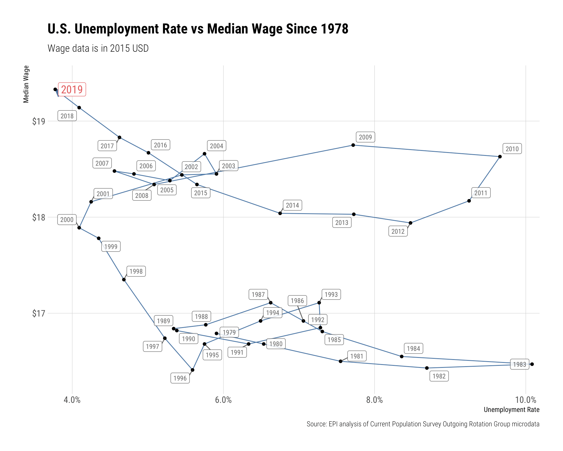
| Lang | # Files | (%) | LoC | (%) | Blank lines | (%) | # Lines | (%) |
|---|---|---|---|---|---|---|---|---|
| R | 18 | 0.47 | 476 | 0.45 | 201 | 0.44 | 490 | 0.47 |
| Rmd | 1 | 0.03 | 58 | 0.05 | 28 | 0.06 | 33 | 0.03 |
| SUM | 19 | 0.50 | 534 | 0.50 | 229 | 0.50 | 523 | 0.50 |
clock Package Metrics for epidata
Please note that this project is released with a Contributor Code of Conduct. By participating in this project you agree to abide by its terms.