
![]()
![]()
![]()
Package ‘ggpmisc’ (Miscellaneous Extensions to ‘ggplot2’) is a set of extensions to R package ‘ggplot2’ (>= 3.0.0) with emphasis on annotations and plotting related to fitted models. Estimates from model fit objects can be displayed in ggplots as text, model equations, ANOVA and summary table. Predicted values, residuals, deviations and weights can be plotted for various model fit functions. Linear models, polynomial regression, quantile regression, major axis regression, non-linear regression and different approaches to robust and resistant regression, as well as user-defined wrapper functions based on them are supported. In addition, all model fit functions returning objects for which accessors are available or supported by package ‘broom’ and its extensions are also supported but not as automatically. Labelling based on multiple comparisons supports various P adjustment methods and contrast schemes. Annotation of peaks and valleys in time series, and scales for volcano and quadrant plots as used for gene expression data are also provided. Package ‘ggpmisc’ continues to give access to extensions moved as of version 0.4.0 to package ‘ggpp’.
Package ‘ggpmisc’ is consistent with the grammar of graphics, and opens new possibilities retaining the flexibility inherent to this grammar. Its aim is not to automate plotting or annotations in a way suitable for fast data exploration by use of a “fits-all-sizes” predefined design. Package ‘ggpmisc’ together with package ‘ggpp’, provide new layer functions, position functions and scales. In fact, these packages follow the tenets of the grammar even more strictly than ‘ggplot2’ in the distinction between geometries and statistics. The new statistics in ‘ggpmisc’ focus mainly on model fitting, including multiple comparisons among groups. The default annotations are those most broadly valid and of easiest interpretation. We follow R’s approach of expecting that users know what they need or want, and will usually want to adjust how results from model fits are presented both graphically and textually. The approach and mechanics of plot construction and rendering remain unchanged from those implemented in package ‘ggplot2’.
Statistics that help with reporting the results of model fits are:
| Statistic | Returned values (default geometry) |
Methods |
|---|---|---|
| Model equation | parameter estimates | |
stat_poly_eq() |
equation, R2,
P, etc. (text_npc) |
lm, rlm, lts, gls, ma, sma, nls, onls, etc. (1, 2, 7) |
stat_ma_eq() |
equation, R2,
P, etc. (text_npc) |
lmodel2 (6, 7) |
stat_quant_eq() |
equation, P, etc.
(text_npc) |
rq (1, 3, 4, 7) |
stat_distrmix_eq() |
equation(s) (text_npc) |
normalmixEM (2, 7) |
stat_correlation() |
correlation, P-value, CI
(text_npc) |
Pearson (t), Kendall (z), Spearman (S) |
stat_fit_glance() |
equation, R2,
P, etc. (text_npc) |
those supported by ‘broom’ |
| Model line | predicted and fitted values | |
stat_poly_line() |
line + conf. (smooth) |
lm, rlm, lts, gls, ma, sma, nls, onls, etc. (1, 2, 7) |
stat_ma_line() |
line + slope conf.
(smooth) |
lmodel2 (6, 7) |
stat_quant_line() |
line + conf. (smooth) |
rq, rqss (1, 3, 4, 7) |
stat_quant_band() |
line + band, 2 or 3 quantiles
(smooth) |
rq, rqss (1, 4, 5, 7) |
stat_distrmix_line() |
lines(s) (line) |
normalmixEM (2, 7) |
stat_fit_augment() |
predicted and other values
(smooth) |
those supported by ‘broom’ |
stat_fit_fitted() |
fitted values (point) |
lm, rlm, lts, rq, gls, ma, sma, nls, onls, etc. (1, 2, 4, 7, 9) |
stat_fit_deviations() |
deviations from observations
(segment) |
lm, rlm, lts, rq, gls, ma, sma, nls, onls, etc. (1, 2, 4, 7, 9) |
| Model table | parameter estimates and significance | |
stat_fit_tb() |
ANOVA and summary tables
(table_npc) |
those supported by ‘broom’ |
stat_fit_tidy() |
fit results, e.g., for equation
(text_npc) |
those supported by ‘broom’ |
| Contrasts | Tukey, Dunnet and arbitrary pairwise | |
stat_multcomp() |
Multiple comparisons
(label_pairwise or text) |
those supported by glht (1,
2, 7) |
| Residuals | model fit residuals | |
stat_fit_residuals() |
residuals (point) |
lm, rlm, lts, rq, gls, ma, sma, nls, onls, etc. (1, 2, 4, 7, 9) |
Notes: (1) weight aesthetic supported; (2) user defined
model fit functions including wrappers of supported methods are accepted
even if they modify the model formula (additional model fitting
methods are likely to work, but have not been tested); (3) unlimited
quantiles supported; (4) user defined fit functions that return an
object of a class derived from rq or rqs are
supported even if they override the statistic’s formula and/or
quantiles argument; (5) two and three quantiles supported; (6)
user defined fit functions that return an object of a class derived from
lmodel2 are supported; (7) method arguments
support colon based notation; (8) model fit functions if method
residuals() defined for returned value; (9) model fit
functions if method fitted() is defined for the returned
value.
Statistics stat_peaks() and stat_valleys()
can be used to highlight and/or label global and/or local maxima and
minima in a plot.
Scales scale_x_logFC(), scale_y_logFC(),
scale_colour_logFC() and scale_fill_logFC()
easy the plotting of log fold change data. Scales
scale_x_Pvalue(), scale_y_Pvalue(),
scale_x_FDR() and scale_y_FDR() are suitable
for plotting p-values and adjusted p-values or false
discovery rate (FDR). Default arguments are suitable for volcano and
quadrant plots as used for transcriptomics, metabolomics and similar
data.
Scales scale_colour_outcome(),
scale_fill_outcome() and scale_shape_outcome()
and functions outome2factor(),
threshold2factor(), xy_outcomes2factor() and
xy_thresholds2factor() used together make it easy to map
ternary numeric outputs and logical binary outcomes to color, fill and
shape aesthetics. Default arguments are suitable for volcano, quadrant
and other plots as used for genomics, metabolomics and similar data.
Several geoms and other extensions formerly included in package
‘ggpmisc’ until version 0.3.9 were migrated to package ‘ggpp’. They are
still available when ‘ggpmisc’ is loaded, but the documentation now
resides in the new package ‘ggpp’.
![]()
Functions for the manipulation of layers in ggplot objects, together
with statistics and geometries useful for debugging extensions to
package ‘ggplot2’, included in package ‘ggpmisc’ until version 0.2.17
are now in package ‘gginnards’.
![]()
library(ggpmisc)
library(ggrepel)
library(broom)
In the first two examples we plot data such that we map a factor to the x aesthetic and label it with the adjusted P-values for multitle comparision using “Tukey” contrasts.
ggplot(mpg, aes(factor(cyl), cty)) +
  geom_boxplot(width = 0.33) +
  stat_multcomp(label.type = "letters") +
  expand_limits(y = 0)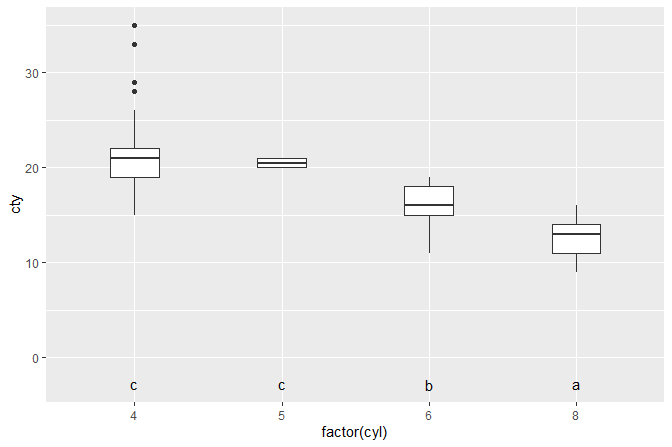
Using “Dunnet” contrasts and “bars” to annotate individual contrasts with the adjusted P-value, here using Holm’s method.
ggplot(mpg, aes(factor(cyl), cty)) +
  geom_boxplot(width = 0.33) +
  stat_multcomp(contrasts = "Dunnet",
                p.adjust.method = "holm",
                size = 2.75) +
  expand_limits(y = 0)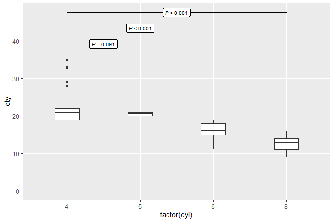
In the third example we add the equation for a linear regression, the
adjusted coefficient of determination and P-value to a plot
showing the observations plus the fitted curve, deviations and
confidence band. We use stat_poly_eq() together with
use_label() to assemble and map the desired
annotations.
formula <- y ~ x + I(x^2)
ggplot(cars, aes(speed, dist)) +
  geom_point() +
  stat_fit_deviations(formula = formula, colour = "red") +
  stat_poly_line(formula = formula) +
  stat_poly_eq(use_label(c("eq", "adj.R2", "P")), formula = formula)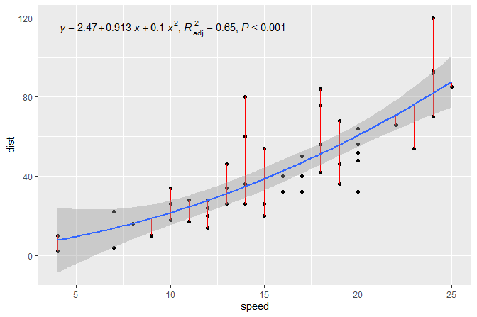
The same figure as in the third example but this time annotated with
the ANOVA table for the model fit. We use stat_fit_tb()
which can be used to add ANOVA or summary tables.
formula <- y ~ x + I(x^2)
ggplot(cars, aes(speed, dist)) +
  geom_point() +
  stat_poly_line(method = "lm", formula = formula) +
  stat_fit_tb(method = "lm",
              method.args = list(formula = formula),
              tb.type = "fit.anova",
              tb.vars = c(Effect = "term",
                          "df",
                          "M.S." = "meansq",
                          "italic(F)" = "statistic",
                          "italic(P)" = "p.value"),
              tb.params = c(x = 1, "x^2" = 2),
              label.y = "top", label.x = "left",
              size = 3.5,
              parse = TRUE)
#> Dropping params/terms (rows) from table!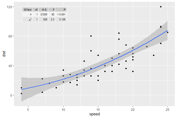
The same figure as in the third example but this time using quantile regression, median in this example.
formula <- y ~ x + I(x^2)
ggplot(cars, aes(speed, dist)) +
  geom_point() +
  stat_quant_line(formula = formula, quantiles = 0.5) +
  stat_quant_eq(use_label("eq", "rho", "n"),
                formula = formula, quantiles = 0.5)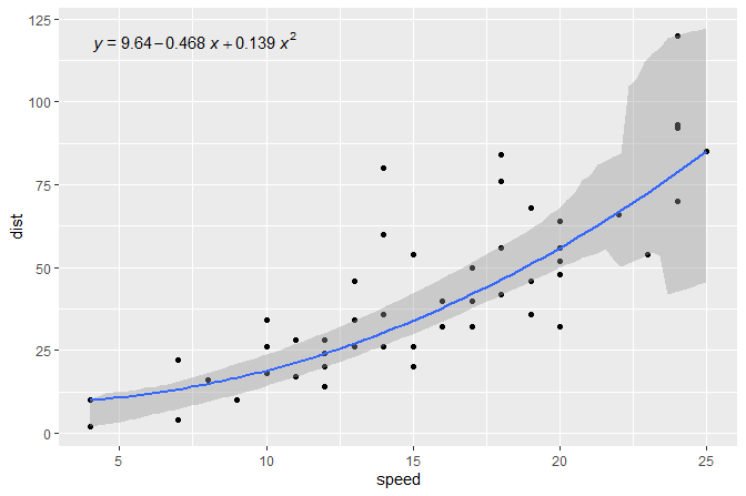
Band highlighting the region between both quartile regressions and a line for the median regression.
formula <- y ~ x + I(x^2)
ggplot(cars, aes(speed, dist)) +
  geom_point() +
  stat_quant_band(formula = formula) +
  stat_quant_eq(formula = formula, quantiles = c(0.25, 0.5, 0.75))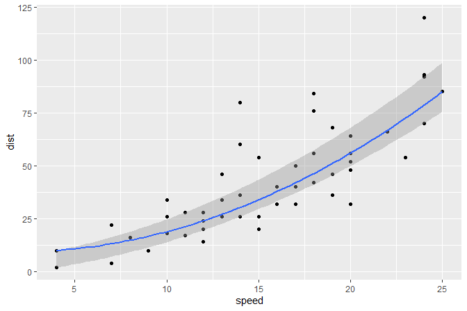
A quadrant plot with counts and labels, using
geom_text_repel() from package ‘ggrepel’.
ggplot(quadrant_example.df, aes(logFC.x, logFC.y)) +
  geom_point(alpha = 0.3) +
  geom_quadrant_lines() +
  stat_quadrant_counts() +
  stat_dens2d_filter(color = "red",
                     keep.fraction = 0.02, h = 3) +
  stat_dens2d_labels(aes(label = gene),
                     keep.fraction = 0.02, h = 3,
                     geom = "text_repel",
                     size = 2,
                     colour = "red") +
  scale_x_logFC(name = "Transcript abundance after A%unit") +
  scale_y_logFC(name = "Transcript abundance after B%unit",
                expand = expansion(mult = 0.2))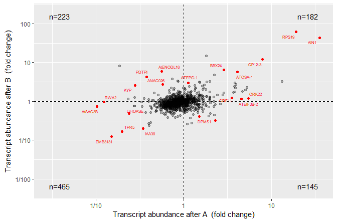
A time series using the specialized version of ggplot()
that converts the time series into a tibble and maps the x
and y aesthetics automatically. We also highlight and label
the peaks using stat_peaks().
ggplot(lynx, as.numeric = FALSE) + geom_line() +
  stat_peaks(colour = "red") +
  stat_peaks(geom = "text", colour = "red", angle = 66,
             hjust = -0.1, x.label.fmt = "%Y") +
  stat_peaks(geom = "rug", colour = "red", sides = "b") +
  expand_limits(y = 8000)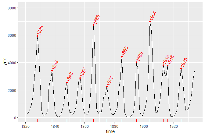
Installation of the most recent stable version from CRAN (sources, Mac and Win binaries):
install.packages("ggpmisc")Installation of the current unstable version from R-Universe CRAN-like repository (binaries for Mac, Win, Webassembly, and Linux, as well as sources available):
install.packages("ggpmisc",
                 repos = c("https://aphalo.r-universe.dev",
                           "https://cloud.r-project.org"))
Installation of the current unstable version from GitHub (from sources):
# install.packages("remotes") # nolint: commented_code_linter.
remotes::install_github("aphalo/ggpmisc")HTML documentation for the package, including help pages and the User Guide, is available at https://docs.r4photobiology.info/ggpmisc/.
News about updates are regularly posted at https://www.r4photobiology.info/.
Chapter 7 in Aphalo (2020) and Chapter 9 in Aphalo (2024) explain basic concepts of the grammar of graphics as implemented in ‘ggplot2’ as well as extensions to this grammar including several of those made available by packages ‘ggpp’ and ‘ggpmisc’. Information related to the book is available at https://www.learnr-book.info/.
Please report bugs and request new features at https://github.com/aphalo/ggpmisc/issues. Pull requests are welcome at https://github.com/aphalo/ggpmisc.
Testing by R-CMD-check.yaml at GitHub is partly
‘ggplot2’-version dependent and run only under the latest R release
because of very small differences in plots and corresponding graphical
“snaps” used as reference. Visual difference tests are never run by CRAN
because they are “fragile” and prone to unexpectedly and spuriously
fail.
If you use this package to produce scientific or commercial publications, please cite according to:
citation("ggpmisc")
#> To cite package 'ggpmisc' in publications use:
#>
#>   Aphalo P (2026). _ggpmisc: Miscellaneous Extensions to 'ggplot2'_. R
#>   package version 1.0.0, <https://docs.r4photobiology.info/ggpmisc/>.
#>
#> A BibTeX entry for LaTeX users is
#>
#>   @Manual{,
#>     title = {ggpmisc: Miscellaneous Extensions to 'ggplot2'},
#>     author = {Pedro J. Aphalo},
#>     year = {2026},
#>     note = {R package version 1.0.0},
#>     url = {https://docs.r4photobiology.info/ggpmisc/},
#> }Being an extension to package ‘ggplot2’, some of the code in package
‘ggpmisc’ has been created by using as a template that from layer
functions and scales in ‘ggplot2’. The user interface of ‘ggpmisc’ aims
at being as consistent as possible with ‘ggplot2’ and the layered
grammar of graphics (Wickham 2010). New features added in ‘ggplot2’ are
added when relevant to ‘ggpmisc’, such as support for
orientation for flipping of layers. This package does
consequently indirectly include significant contributions from several
of the authors and maintainers of ‘ggplot2’, listed at (https://ggplot2.tidyverse.org/).
Aphalo, Pedro J. (2024) Learn R: As a Language. 2ed. The R Series. Boca Raton and London: Chapman and Hall/CRC Press. ISBN: 9781032516998. 466 pp.
Aphalo, Pedro J. (2020) Learn R: As a Language. 1ed. The R Series. Boca Raton and London: Chapman and Hall/CRC Press. ISBN: 9780367182533. 350 pp.
Wickham, Hadley. 2010. “A Layered Grammar of Graphics.” Journal of Computational and Graphical Statistics 19 (1): 3–28. https://doi.org/10.1198/jcgs.2009.07098.
© 2016-2026 Pedro J. Aphalo (pedro.aphalo@helsinki.fi). Released under the GPL, version 2 or greater. This software carries no warranty of any kind.