 The
resulting variogram model (
The
resulting variogram model (gsm.f$model in case of a “gstat”
object) can the be appended to the spatial model, withThe goal of gmGeostats is to provide a unified framework for the geostatistical analysis of multivariate data from any statistical scale, e.g. data honoring a ratio scale, or with constraints such as spherical or compositional data.
This R package offers support for geostatistical analysis of multivariate data, in particular data with restrictions, e.g. positive amounts data, compositional data, distributional data, microstructural data, etc. It includes descriptive analysis and modelling for such data, both from a two-point Gaussian perspective and multipoint perspective. The package is devised for supporting 3D, multi-scale and large data sets and grids. This is a building block of the suite of HIF geometallurgical software.
You can install the released version of gmGeostats from CRAN with:
install.packages("gmGeostats")Read the package vignette for an extended scheme of the package functionality. The fundamental steps are:
## load the package (NOTE: do not load "compositions" or "gstat" afterwards!)
library(gmGeostats)
#> Welcome to 'gmGeostats', a package for multivariate geostatistical analysis.
#>  Note: use 'fit_lmc' instead of fit.lmc

## read your data, identify coordinates and sets of variables
data("Windarling") # use here some read*(...) function
colnames(Windarling)
#>  [1] "Hole_id"     "Sample.West" "Sample.East" "West"        "East"
#>  [6] "Easting"     "Northing"    "Lithotype"   "Fe"          "P"
#> [11] "SiO2"        "Al2O3"       "S"           "Mn"          "CL"
#> [16] "LOI"
X = Windarling[,c("Easting", "Northing")]
Z = Windarling[,c(9:12,14,16)]

## declare the scale of each set of variables
Zc = compositions::acomp(Z) # other scales will come in the future

## pack the data in a gmSpatialModel object using an appropriate
#     make.** function
gsm = make.gmCompositionalGaussianSpatialModel(
  data = Zc, coords = X, V = "alr", formula = ~1
)
From this point on, what you do depends on which model do you have in
mind. Here we briefly cover the case of a Gaussian model, though a
multipoint approach can also be tackled with function
make.gmCompositionalMPSSpatialModel() providing a training
image as model. See the package vignette for details.
A structural analysis can be obtained in the following steps
## empirical structural function
vge = variogram(gsm)
## model specification
vm = gstat::vgm(model="Sph", range=25, nugget=1, psill=1)
# you can use gstat specifications!
## model fitting
gsm.f = fit_lmc(v = vge, g = gsm, model = vm)
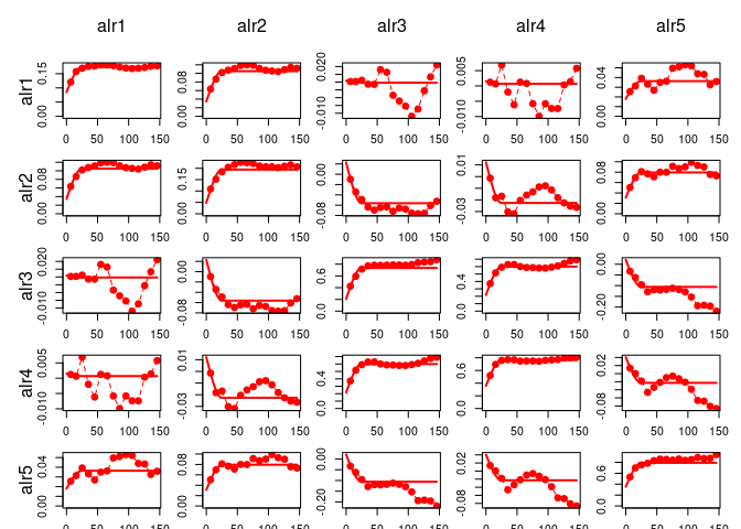
## plot
variogramModelPlot(vge, model = gsm.f, col="red") The
resulting variogram model (gsm.f$model in case of a “gstat”
object) can the be appended to the spatial model, with
gsm = make.gmCompositionalGaussianSpatialModel(
  data = Zc, coords = X, V = "alr", formula = ~1,
  model = gsm.f$model
)
Other empirical structural functions (e.g. logratio variograms from
package “compositions”) and their theoretical counterparts
(e.g. “CompLinModCoReg” objects from “compositions” or “LMCAnisCompo”
from “gmGeostats”) can also be estimated resp. fitted and given to the
argument model of this call to
make.gmCompositionalGaussianSpatialModel. Other additional
arguments are the mean value in case of simple (co)kriging, or
descriptors of the local neighbourhood (see
?make.gmCompositionalGaussianSpatialModel for more
information), both using the same parameter names as in
?gstat::gstat for ease of use.
The resulting geostatistical model (including conditioning data and structural model) can then be validated, interpolated and/or simulated. The workflow for each of these tasks is always:
1.- define some method parameters with a tailored function,
e.g. LeaveOneOut() for validation,
KrigingNeighbourhood() for cokriging (the neighbourgood can
also be appended to make.*SpatialModel()-calls) or
SequentialSimulation() for sequential Gaussian
Simulation
2.- if desired, define some new locations where to interpolate or
simulate, using expand.grid(),
sp::GridTopology() or alternatives from other packages
3.- call an appropriate analysis function, specifying the model,
potential new data, and the parameters created in the preceding steps;
e.g. validate(model, pars) for validation, or
predict(model, newdata, pars) for interpolation or
simulation
More information can be found in the package vignette.