
The goal of ham is to provide different modeling approaches to evaluating healthcare programs (or programs in other fields) with regression analysis. This includes standard regression methods like linear (OLS) and logistic regression. And ham adds options for differences-in-differences models as well as interrupted time-series analysis. DID and ITS models offer options for causal modeling. What is unique about ham is that it creates datasets with constructed variables for DID and ITS models, optionally it can add top coded outcome variables, propensity scores, and provides some interpretation of model results. Additionally, Cronbach’s alpha can be calculated for such things as patient surveys. As the logo of Dr. Ham suggests, the ham package can help illuminate your results.
You can install the development version of ham from GitHub with:
# install.packages("devtools")
devtools::install_github("szuniga07/ham")An example of calculating Cronbach’s alpha:
library(ham)
alpha(items=c("i1","i2","i3","i4","i5"), data=cas)
#> Scale statistics
#> Cronbach's alpha   = 0.919
#> Mean               = 3.772
#> Variance           = 0.453
#> Standard Deviation = 0.673
#> Items              = 5
#>
#> Item statistics
#>    Mean Variance Std. Dev.
#> i1 3.50    0.434     0.659
#> i2 3.81    0.681     0.825
#> i3 3.88    0.652     0.808
#> i4 3.82    0.594     0.770
#> i5 3.85    0.634     0.796
#>
#> Scale statistics if item deleted
#>    Alpha  Mean Variance Std. Dev.
#> i1 0.930 3.840    0.528     0.727
#> i2 0.891 3.763    0.436     0.660
#> i3 0.883 3.745    0.433     0.658
#> i4 0.910 3.760    0.472     0.687
#> i5 0.885 3.752    0.439     0.662
#>
#> Sample
#> Total    = 100
#> Valid    = 100
#> Excluded = 0

## Interpret the results
interpret(alpha(items=c("i1","i2","i3","i4","i5"), data=cas))
#> Interpretations: Alpha
#> ----------------------
#> Your 5 item scale has a Cronbach's alpha of 0.919. This is
#> generally considered as being in the 'excellent' range.
#>
#> The scale mean is 3.77 and has a standard deviation of 0.673.
#>
#> Removing one of these item(s): i1, can improve the Cronbach's
#> alpha in a new scale to a higher level than the current alpha
#> based on all items.
#>
#> 0 row(s) of data excluded from the analysis because of missing
#> data.This is the ham package on healthcare analysis methods. This package can help when performing program evaluations or intervention studies in healthcare. Or simply to test if a program has an impact on an outcome of interest.
ham can help with research or evaluation studies. When working in healthcare systems, multi-site evaluations can strongly resemble research studies and commonly use regression methods. For an introduction to evaluation, please see the reference below.
Patton, M. Q. (1997). Utilization-focused evaluation: The new century text (3rd ed.). Thousand Oaks, CA: Sage Publications
What is unique about ham, is that it provides options for running standard linear or ordinary least squares (OLS) and logistic regression as well as methods used in causal modeling such as differences-in-differences (DID) and interrupted time series analysis (ITS). It also optionally makes data with the newly created variables (i.e., this saves you time).
This vignette will introduce ham’s features in the following functions: * alpha: Conduct Cronbach’s alpha on scale items (e.g., survey questions). * assess: Perform various regression methods (OLS, logistic, differences-in-differences, and interrupted time series) * importance: Rank variable importance from regression coefficients using the partial chi-square statistic. * interpret: Provides simple coefficient interpretations. This is a helpful reminder, especially as models have increased coefficients (e.g., ITS). * There are also printing and plotting options to help review your results.
Below will cover 3 sections with examples of the different features along the way.
This example shows group level point estimates and confidence intervals. There is also an option to retrieve those estimates over time periods. And there are graphing options to help see how the data looks for both.
Results can be returned for each unit of time, as increments such as for each 3 months (i.e., quarters) or for rolling averages such as a rolling 12-month period. Using increments of multiple months or as rolling averages can help visualize results when there is high variation over time.
gr1 <- group(x="program", y="los", z="month", data=hosprog, dist="t", increment=3, rolling=6)
print(gr1$Group.CI)
#> $adf_alpha
#>   Group PointEst    Lower    Upper
#> 1     1 4.247012 4.034842 4.459181
#> 0     0 4.585967 4.391132 4.780802
#>
#> $adf_numeric
#>   Group PointEst    Lower    Upper
#> 0     0 4.585967 4.391132 4.780802
#> 1     1 4.247012 4.034842 4.459181
#>
#> $adf_all
#>   PointEst    Lower    Upper
#> 1 4.428259 4.284543 4.571974plot(x=gr1, y="group", order="numeric", lwd=4, gcol= "blue", pcol="red", overall=TRUE, oband=TRUE, ocol="gray", tcol="green", tgt=4.5, cex=2, cex.axis=1, cex.lab=1.1, cex.text=2, cex.main=1.25, adj.alpha=.2)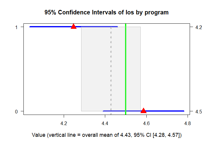
plot(x=gr1, y="time", lwd=4, gcol=c("red", "blue"), gband=TRUE, overall=TRUE, oband=TRUE, ocol="gray", tcol="green", tgt=4, tpline=3, tpcol="yellow", name=TRUE, cex.axis=1, cex.lab=1, cex.text=2, cex.main=1.25, adj.alpha=.3)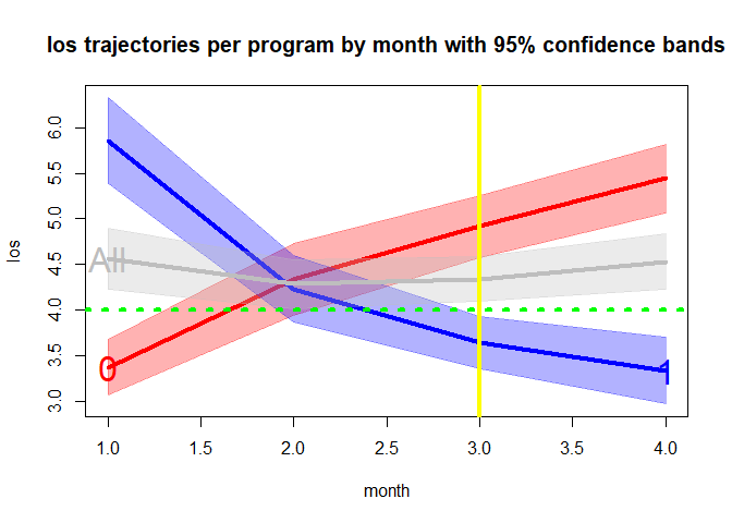
The example dataset has common variables found in program evaluation or intervention studies (I’ll refer to both as a ‘study’), there are various outcome and predictor variables (or response and explanatory variables or dependent and independent variables or other names common in your field). In these studies, we try to assess the impact of the predictors on the outcome. We often use treatment and control groups to asses a healthcare program or intervention’s impact on our key outcome variable of interest. Because of multiple stakeholders, we often conduct these studies with multiple outcomes to help answer the multiple stakeholder’s questions.
A common approach to answering study questions is using a regression to test a treatment effect while controlling for other covariates.
Here are OLS and logistic regression example using assess() on the mtcars data. These use lm() and glm() found in R’s stats package.
summary(assess(hp ~ mpg+wt, data=mtcars, regression="ols")$model)
#>
#> Call:
#> stats::lm(formula = primary_formula, data = combined_df, weights = wght_obj,
#>     offset = offst_obj)
#>
#> Residuals:
#>    Min     1Q Median     3Q    Max
#> -59.42 -30.75 -12.07  24.82 141.84
#>
#> Coefficients:
#>             Estimate Std. Error t value Pr(>|t|)
#> (Intercept)  349.287    103.509   3.374  0.00212 **
#> mpg           -9.417      2.676  -3.519  0.00145 **
#> wt            -4.168     16.485  -0.253  0.80217
#> ---
#> Signif. codes:  0 '***' 0.001 '**' 0.01 '*' 0.05 '.' 0.1 ' ' 1
#>
#> Residual standard error: 44.65 on 29 degrees of freedom
#> Multiple R-squared:  0.6033, Adjusted R-squared:  0.576
#> F-statistic: 22.05 on 2 and 29 DF, p-value: 1.505e-06summary(assess(formula=vs~mpg+wt+hp, data=mtcars, regression="logistic")$model)
#>
#> Call:
#> stats::glm(formula = primary_formula, family = binomial(link = family_link),
#> data = combined_df, weights = wght_obj, offset = offst_obj)
#>
#> Coefficients:
#> Estimate Std. Error z value Pr(>|z|)
#> (Intercept) -10.61945 16.52453 -0.643 0.5205
#> mpg 0.50291 0.48656 1.034 0.3013
#> wt 3.87749 3.19255 1.215 0.2245
#> hp -0.09318 0.04318 -2.158 0.0309 *
#> ---
#> Signif. codes: 0 '***' 0.001 '**' 0.01 '*' 0.05 '.' 0.1 ' ' 1
#>
#> (Dispersion parameter for binomial family taken to be 1)
#>
#> Null deviance: 43.860 on 31 degrees of freedom
#> Residual deviance: 14.748 on 28 degrees of freedom
#> AIC: 22.748
#>
#> Number of Fisher Scoring iterations: 8
## Interpret the results
interpret(assess(formula=vs~mpg+wt+hp, data=mtcars, regression="logistic")
)$model
#> Interpretations: Regression model
#> ---------------------------------
#> These estimates tell you about the relationship between the
#> independent variables and the dependent variable. These estimates
#> tell the amount of change in outcome scores that would be
#> predicted by a 1 unit increase in the predictor.
#>
#> The following predictor variable(s) have coefficient(s)
#> significantly different from 0 using an alpha of 0.05:
#> hp
#>
#> For every 1 unit increase in these predictor variables,
#> vs is predicted to increase by the value of the
#> coefficient, holding all other variables constant. The following
#> predictor variable(s) have positive coefficient(s) that
#> increase the predicted value and odds of the outcome:
#> No positive coefficients in your model were significant.
#>
#> For every 1 unit increase in these predictor variables,
#> vs is predicted to decrease by the value of the
#> coefficient, holding all other variables constant. The following
#> predictor variable(s) have negative coefficient(s) that
#> decrease the predicted value and odds of the outcome:
#> hp (8.9% decreased odds)
#>
#> C-statistic/AUC. The probability of concordance is identical
#> to the AUC. It computes all possible pairs of subjects
#> (response=1 vs. response=0). The index is the proportion of such
#> pairs with the responder having a higher predicted probability of
#> response than the nonresponder. The C-statistic/AUC is 0.956.m04 <- assess(formula=HAI ~ Month+ offset(log(PatientDays)),
data=infections, regression="poisson")
#Because 1 year is a meaningful period in program evaluation, Month=12
plot(x=review(m04$model, increase=c(Month=12)), xlim=c(0.6, 1.01),
lwd=7, color="cyan", pcol="salmon", pt.cex=2)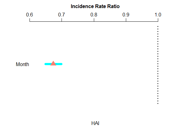
ham can topcode the outcome and create a propensity score variable. Here is an example using the artificially created hosprog data with hospital stay cost as the outcome with a novel hospital program/intervention binary indicator and a 12 month time variable. The option for new data being returned is specified with newdata=TRUE.
top coding cost at $17,150 and propensity score based on age, female indicator, and a health risk probability score.
m1 <- assess(formula=cost ~ month * program, data=hosprog, intervention = "program",
regression="ols", topcode=17150, propensity=c("female","age","risk"),
newdata=TRUE)summary(m1$model)
#>
#> Call:
#> stats::lm(formula = primary_formula, data = combined_df, weights = wght_obj,
#> offset = offst_obj)
#>
#> Residuals:
#> Min 1Q Median 3Q Max
#> -6570.9 -2158.3 -598.1 1962.0 10521.1
#>
#> Coefficients:
#> Estimate Std. Error t value Pr(>|t|)
#> (Intercept) 14006.64 1363.65 10.271 < 2e-16 ***
#> month 424.81 46.57 9.122 < 2e-16 ***
#> program 5524.74 514.18 10.745 < 2e-16 ***
#> pscore -15989.00 2838.57 -5.633 2.55e-08 ***
#> month:program -908.68 68.64 -13.239 < 2e-16 ***
#> ---
#> Signif. codes: 0 '***' 0.001 '**' 0.01 '*' 0.05 '.' 0.1 ' ' 1
#>
#> Residual standard error: 3165 on 715 degrees of freedom
#> Multiple R-squared: 0.233, Adjusted R-squared: 0.2287
#> F-statistic: 54.3 on 4 and 715 DF, p-value: < 2.2e-16Descriptive statistics on newly created variables and the original cost as a comparison. top.cost is the topcoded cost variable.
summary(m1$newdata[, c( "cost","top.cost", "pscore")])
#>       cost          top.cost         pscore
#>  Min.   : 1483   Min.   : 1483   Min.   :0.3708
#>  1st Qu.: 6410   1st Qu.: 6410   1st Qu.:0.4364
#>  Median : 8639   Median : 8639   Median :0.4655
#>  Mean   : 9348   Mean   : 9215   Mean   :0.4653
#>  3rd Qu.:11487   3rd Qu.:11487   3rd Qu.:0.4942
#> Max. :27540 Max. :17150 Max. :0.5609We can examine variable importance based on partial chi-square (i.e., which variables explain the outcome the most).
importance(m1$model)
#>               X    Chi.Sq d.f.      p.value
#> 1         month 175.30630    2 8.564878e-39
#> 2       program 179.92844    2 8.492485e-40
#> 3        pscore  31.72813    1 1.773352e-08
#> 4 month:program 175.27159 1 5.222734e-40We can examine variable importance to see a ranking of variables with a graph. The hospital program has the highest rank, variables highlighted in red are statistically significant.
#Consider using these graphical parameters
par(mar=c(4.2, 2, 3.5, 3))
par(oma = c(0, 0, 0, 3))
plot(importance(m1$model))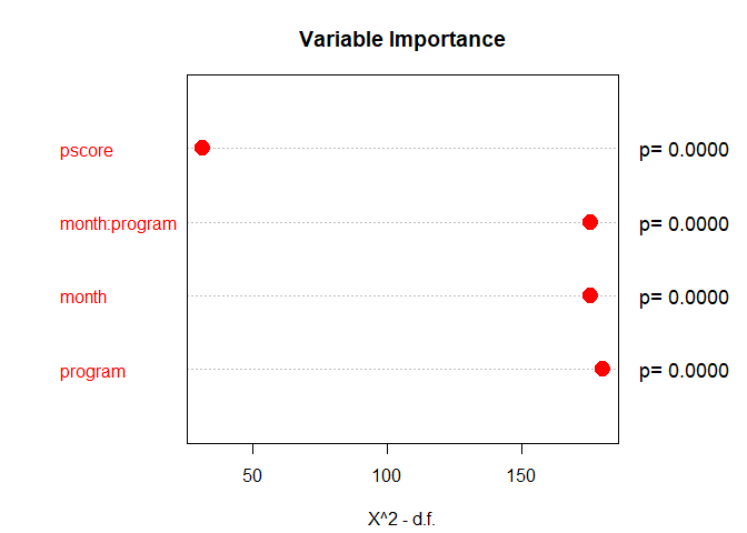
Topcoding can be applied to any model. Propensity scores can be created for any model except the single group interrupted time series because there is no control group (i.e. intervention group only).
DID can be used on binary or continuous outcome variables. Below is an example using the hosprog data with length of stay as the outcome and the created DID variables as the predictors, use ‘.’ on the right-hand side of the formula to indicate only the created variables will be used. Replace ‘.’ with any additional selected variables. The newly created DID variables will be added in all DID models. This model has a pre/post design (i.e., there are only 2 distinct time points) by selecting: did=“two”, with post starting at month 5.
dm1 <- assess(formula= los ~ ., data=hosprog, intervention = "program",
int.time="month", treatment= 5, did="two")summary(dm1$DID)
#>
#> Call:
#> stats::lm(formula = DID_formula, data = combined_df, weights = wght_obj,
#> offset = offst_obj)
#>
#> Residuals:
#> Min 1Q Median 3Q Max
#> -3.6247 -1.2003 -0.3145 0.8564 8.8642
#>
#> Coefficients:
#> Estimate Std. Error t value Pr(>|t|)
#> (Intercept) 3.4940 0.1650 21.175 < 2e-16 ***
#> Post.All 1.5629 0.1974 7.917 9.25e-15 ***
#> Int.Var 2.0664 0.2349 8.797 < 2e-16 ***
#> DID -3.5448 0.2849 -12.444 < 2e-16 ***
#> ---
#> Signif. codes: 0 '***' 0.001 '**' 0.01 '*' 0.05 '.' 0.1 ' ' 1
#>
#> Residual standard error: 1.777 on 716 degrees of freedom
#> Multiple R-squared: 0.1848, Adjusted R-squared: 0.1814
#> F-statistic: 54.11 on 3 and 716 DF, p-value: < 2.2e-16interpret(dm1)$did
#> Interpretations: DID
#> --------------------
#> The intercept represents the mean los value of the
#> control group at the baseline period (Time 1): 3.49.
#>
#> Post.All is the change in the control group's los
#> value in the 2nd time period (Time 2). There is a
#> significant increase for the control group
#> at time 2: 1.56.
#>
#> Int.Var is the difference between the intervention
#> and control group at the baseline period (Time 1). The
#> intervention group had a significant increase in the
#> mean los value compared to the control group: 2.07.
#>
#> DID estimates the average treatment effect on the
#> treated group (ATET). This interaction represents the
#> difference in the trend differences for the intervention and
#> control groups:
#> (Int. Time 2 - Int. Time 1) - (Ctl. Time 2 - Ctl. Time 1) = -3.54.
#> In other words, there is a significant decrease in the
#> mean los trend by -3.54 for the intervention group.
#>
#> If there are additional variables in the model then the coefficients
#> above represent the effects after controlling for the other variables.
#>
#> R-Squared (R2) is the proportion of variance in the dependent
#> variable which can be predicted from the independent
#> variable(s). For example, if R2 = 0.50, 50% of the variance
#> in test scores can be predicted from the 5 variables. R2 >= 0.80
#> may be at a level to reliably make individual predictions.
#> Lower R2 may be helpful in group level predictions. And low R2 can
#> still be adequate for hypothesis testing. The R2 is 0.185.This model allows for more than 2 time points. It allows for monthly increments by selecting did=“many”.
dm2 <- assess(formula= los ~ ., data=hosprog, intervention = "program",
int.time="month", treatment= 5, did="many")summary(dm2$DID)
#>
#> Call:
#> stats::lm(formula = DID_formula, data = combined_df, weights = wght_obj,
#> offset = offst_obj)
#>
#> Residuals:
#> Min 1Q Median 3Q Max
#> -3.7149 -1.2747 -0.3732 0.8838 9.1718
#>
#> Coefficients:
#> Estimate Std. Error t value Pr(>|t|)
#> (Intercept) 4.17164 0.16049 25.994 < 2e-16 ***
#> Period 0.10837 0.02342 4.627 4.4e-06 ***
#> DID 0.14843 0.48630 0.305 0.760284
#> DID.Trend -0.19580 0.05712 -3.428 0.000643 ***
#> ---
#> Signif. codes: 0 '***' 0.001 '**' 0.01 '*' 0.05 '.' 0.1 ' ' 1
#>
#> Residual standard error: 1.853 on 716 degrees of freedom
#> Multiple R-squared: 0.1135, Adjusted R-squared: 0.1098
#> F-statistic: 30.57 on 3 and 716 DF, p-value: < 2.2e-16interpret(dm2)$did
#> Interpretations: DID
#> --------------------
#> The intercept represents the starting point of the control
#> group's trend line at the baseline period (Time 1): 4.17.
#>
#> Period is the change in the control group's los value trend
#> line after the baseline period. There is a significant increase
#> for the control group after the baseline period: 0.108.
#>
#> DID estimates the difference in mean overall level between
#> the intervention and both the non-intervention period/group.
#> In other words, there is a non-significant increase in the
#> mean los by 0.148 for the intervention group.
#>
#> DID.Trend is the difference in the intervention group's
#> trend line after the intervention period started (> Time 1).
#> The intervention group had a significant decrease in trend
#> of the mean los by -0.196 after the intervention started.
#>
#> If there are additional variables in the model then the coefficients
#> above represent the effects after controlling for the other variables.
#>
#> R-Squared (R2) is the proportion of variance in the dependent
#> variable which can be predicted from the independent
#> variable(s). For example, if R2 = 0.50, 50% of the variance
#> in test scores can be predicted from the 5 variables. R2 >= 0.80
#> may be at a level to reliably make individual predictions.
#> Lower R2 may be helpful in group level predictions. And low R2 can
#> still be adequate for hypothesis testing. The R2 is 0.114.We can also use DID on binary outcomes like hospital re-admission within 30-days.
dm3 <- assess(formula= rdm30 ~ ., data=hosprog, intervention = "program",
int.time="month", treatment= 5, did="two")summary(dm3$DID)
#>
#> Call:
#> stats::lm(formula = DID_formula, data = combined_df, weights = wght_obj,
#> offset = offst_obj)
#>
#> Residuals:
#> Min 1Q Median 3Q Max
#> -0.31858 -0.25651 -0.07207 -0.06034 0.93966
#>
#> Coefficients:
#> Estimate Std. Error t value Pr(>|t|)
#> (Intercept) 0.06034 0.03422 1.763 0.0782 .
#> Post.All 0.19616 0.04094 4.792 2.01e-06 ***
#> Int.Var 0.25824 0.04871 5.301 1.53e-07 ***
#> DID -0.44267 0.05907 -7.493 1.98e-13 ***
#> ---
#> Signif. codes: 0 '***' 0.001 '**' 0.01 '*' 0.05 '.' 0.1 ' ' 1
#>
#> Residual standard error: 0.3686 on 716 degrees of freedom
#> Multiple R-squared: 0.0759, Adjusted R-squared: 0.07203
#> F-statistic: 19.6 on 3 and 716 DF, p-value: 3.197e-12Significant DID effect showing reduced re-admissions
ITS lets us look at trends for 1 or 2 groups such as an intervention/treatment group without a control group or both a treatment and control group. And we have the option of one or more treatment periods (or interruptions). This gives us 4 options that can be specified using the interrupt and its= arguments.
Below are examples using the hosprog data for the patient length of stay (LOS) and death within 30-days. The dataset hosp1 will be used for the single group examples.
We begin by looking at a single group with a single interruption/treatment period and assessing their LOS scores. We specify it with: interrupt= 5 and its=“one”.
im11 <- assess(formula=los ~ ., data=hosp1, intervention = "program",
int.time="month", interrupt= 5, its="one")summary(im11$ITS)
#>
#> Call:
#> stats::lm(formula = ITS_formula, data = combined_df, weights = wght_obj,
#> offset = offst_obj)
#>
#> Residuals:
#> Min 1Q Median 3Q Max
#> -3.7673 -1.1321 -0.3755 0.5758 9.1718
#>
#> Coefficients:
#> Estimate Std. Error t value Pr(>|t|)
#> (Intercept) 6.3299 0.4170 15.178 <2e-16 ***
#> ITS.Time -0.2889 0.1442 -2.003 0.0460 *
#> post5 -1.0026 0.4264 -2.351 0.0193 *
#> txp5 0.2014 0.1522 1.324 0.1865
#> ---
#> Signif. codes: 0 '***' 0.001 '**' 0.01 '*' 0.05 '.' 0.1 ' ' 1
#>
#> Residual standard error: 1.726 on 331 degrees of freedom
#> Multiple R-squared: 0.2426, Adjusted R-squared: 0.2357
#> F-statistic: 35.34 on 3 and 331 DF, p-value: < 2.2e-16interpret(im11)$its
#> Interpretations: ITS
#> --------------------
#> Note: Some variable names below based on time points (or 'interruptions').
#> This analysis is for a one-group, single intervention period (interruption).
#>
#> Intercept is 6.33 and the starting value of the trend
#> for the intervention group.
#>
#> ITS.Time is -0.289 and the slope prior to intervention.
#> The coefficient is significant.
#>
#> post5 is -1 and the immediate shift in the trend line
#> after the intervention start (e.g., 1st year of intervention).
#> The coefficient is significant.
#>
#> txp5 is 0.201 and the difference between pre- and
#> post-intervention slopes (e.g., change in the pre-intervention
#> slope). The coefficient is non-significant.
#>
#> Summary: The results show that after the start of the intervention,
#> there is a non-significant change in the los trend. This gives
#> a post-intervention trend change per time unit in the los of -0.0874
#> (i.e., the value of change per-unit-of-time, such as month or year, in
#> the intervention period; not the change relative to pre-intervention).
#>
#> If there are additional variables in the model then the coefficients
#> above represent effects after controlling for the other variables.
#>
#> R-Squared (R2) is the proportion of variance in the dependent
#> variable which can be predicted from the independent
#> variable(s). For example, if R2 = 0.50, 50% of the variance
#> in test scores can be predicted from the 5 variables. R2 >= 0.80
#> may be at a level to reliably make individual predictions.
#> Lower R2 may be helpful in group level predictions. And low R2 can
#> still be adequate for hypothesis testing. The R2 is 0.243.‘Summary’ reviews the results but in order to view the point estimate and confidence interval, check the results with the itsEffect function. This also provides the standard error, t-statistic, and p-value. Just specify the model type= “sgst” and interruptions= 1 for a single-group, single time period analysis with 1 interruption.
itsEffect(model= im11$ITS, type= "sgst", interruptions= 1)
#>                   Effect       S.E.         t    p.value        L95         U95
#> Intervention -0.08743239 0.04851635 -1.802122 0.07243586 -0.1828716 0.008006875
There is a second key period of interest at month 9 which is specified with interrupt= c(5, 9) and its=“one”
im12 <- assess(formula=los ~ ., data=hosp1, intervention = "program",
int.time="month", interrupt= c(5, 9), its="one")summary(im12$ITS)
#>
#> Call:
#> stats::lm(formula = ITS_formula, data = combined_df, weights = wght_obj,
#> offset = offst_obj)
#>
#> Residuals:
#> Min 1Q Median 3Q Max
#> -3.7673 -1.1571 -0.2641 0.5841 8.8966
#>
#> Coefficients:
#> Estimate Std. Error t value Pr(>|t|)
#> (Intercept) 6.3299 0.4157 15.226 <2e-16 ***
#> ITS.Time -0.2889 0.1438 -2.009 0.0453 *
#> post5 -0.9877 0.4569 -2.161 0.0314 *
#> txp5 0.2517 0.2051 1.227 0.2207
#> post9 -0.7806 0.5100 -1.530 0.1269
#> txp9 0.2296 0.2114 1.086 0.2781
#> ---
#> Signif. codes: 0 '***' 0.001 '**' 0.01 '*' 0.05 '.' 0.1 ' ' 1
#>
#> Residual standard error: 1.72 on 329 degrees of freedom
#> Multiple R-squared: 0.2519, Adjusted R-squared: 0.2405
#> F-statistic: 22.16 on 5 and 329 DF, p-value: < 2.2e-16We continue with comparing the intervention and control groups on their LOS scores which is specified with interrupt= 5 and its=“two”.
im21 <- assess(formula=los ~ ., data=hosprog, intervention = "program",
int.time="month", interrupt= 5, its="two")summary(im21$ITS)
#>
#> Call:
#> stats::lm(formula = ITS_formula, data = combined_df, weights = wght_obj,
#> offset = offst_obj)
#>
#> Residuals:
#> Min 1Q Median 3Q Max
#> -3.7673 -1.1722 -0.3348 0.8794 9.1718
#>
#> Coefficients:
#> Estimate Std. Error t value Pr(>|t|)
#> (Intercept) 3.0896 0.3951 7.821 1.90e-14 ***
#> ITS.Time 0.1635 0.1455 1.123 0.2617
#> ITS.Int 3.2403 0.5790 5.596 3.13e-08 ***
#> txi -0.4523 0.2064 -2.191 0.0287 *
#> post5 0.4413 0.4508 0.979 0.3279
#> txp5 0.0297 0.1530 0.194 0.8462
#> ixp5 -1.4439 0.6249 -2.311 0.0211 *
#> txip5 0.1717 0.2174 0.790 0.4299
#> ---
#> Signif. codes: 0 '***' 0.001 '**' 0.01 '*' 0.05 '.' 0.1 ' ' 1
#>
#> Residual standard error: 1.752 on 712 degrees of freedom
#> Multiple R-squared: 0.2124, Adjusted R-squared: 0.2046
#> F-statistic: 27.43 on 7 and 712 DF, p-value: < 2.2e-16We have an interest in a 2nd interruption at month 9, which is specified with interrupt= c(5, 9) and its=“two”.
im22 <- assess(formula=los ~ ., data=hosprog, intervention = "program",
int.time="month", interrupt= c(5, 9), its="two")summary(im22$ITS)
#>
#> Call:
#> stats::lm(formula = ITS_formula, data = combined_df, weights = wght_obj,
#> offset = offst_obj)
#>
#> Residuals:
#> Min 1Q Median 3Q Max
#> -3.7673 -1.1755 -0.2888 0.9020 8.8966
#>
#> Coefficients:
#> Estimate Std. Error t value Pr(>|t|)
#> (Intercept) 3.08956 0.39418 7.838 1.68e-14 ***
#> ITS.Time 0.16346 0.14519 1.126 0.2606
#> ITS.Int 3.24031 0.57773 5.609 2.92e-08 ***
#> txi -0.45232 0.20594 -2.196 0.0284 *
#> post5 0.59672 0.47463 1.257 0.2091
#> txp5 -0.03780 0.20378 -0.186 0.8529
#> ixp5 -1.58438 0.66393 -2.386 0.0173 *
#> txip5 0.28951 0.29147 0.993 0.3209
#> post9 -0.21293 0.46895 -0.454 0.6499
#> txp9 0.28005 0.19285 1.452 0.1469
#> ixp9 -0.56762 0.69886 -0.812 0.4169
#> txip9 -0.05043 0.28863 -0.175 0.8613
#> ---
#> Signif. codes: 0 '***' 0.001 '**' 0.01 '*' 0.05 '.' 0.1 ' ' 1
#>
#> Residual standard error: 1.748 on 708 degrees of freedom
#> Multiple R-squared: 0.2203, Adjusted R-squared: 0.2081
#> F-statistic: 18.18 on 11 and 708 DF, p-value: < 2.2e-16interpret(im22)$its
#> Interpretations: ITS
#> --------------------
#> Note: Some variable names below based on time points (or 'interruptions').
#> This analysis is for a two-group, multiple intervention period (interruption).
#> Positive values indicate higher intervention group values and vice-versa for:
#> Coefficients that begin with 'post', 'txp', 'ixp', and 'txip'.
#>
#> Intercept is 3.09 and the starting value of the trend for the
#> control group.
#>
#> ITS.Time is 0.163 and the control group's slope prior to intervention.
#> The coefficient is non-significant.
#>
#> ITS.Int is 3.24 and the difference in the level between intervention
#> and control group prior to intervention 1 (intervention - control).
#> The coefficient is significant.
#>
#> txi is -0.452 and the difference between the intervention and
#> control group's pre-intervention slopes (intervention - control).
#> The coefficient is significant.
#>
#> post5 is 0.597 and the immediate shift in the control group trend
#> line after this intervention time starts. The coefficient is
#> non-significant.
#>
#> txp5 is -0.0378 and the difference between current and prior intervention
#> control group slopes (e.g., change in the pre-intervention slope).
#> The coefficient is non-significant.
#>
#> ixp5 is -1.58 and the difference between the intervention and
#> control groups (intervention - control) in the period immediately
#> after this intervention started (e.g., 1st year of intervention 1).
#> The coefficient is significant.
#>
#> txip5 is 0.29 and non-significant. This is the difference in both
#> group's slope changes since the prior intervention (pre-slopes compared
#> to post-slopes). For example, both have pre-intervention slopes
#> of 2, the control group's slope remained the same, therefore the
#> post 1st intervention slope is 0. And the intervention group's slope
#> increased by 2, then txip1 = 2 (= 2 - 0).
#>
#> post9 is -0.213 and the immediate shift in the control group trend
#> line after this intervention time starts. The coefficient is
#> non-significant.
#>
#> txp9 is 0.28 and the difference between current and prior intervention
#> control group slopes (e.g., change in the pre-intervention slope).
#> The coefficient is non-significant.
#>
#> ixp9 is -0.568 and the difference between the intervention and
#> control groups (intervention - control) in the period immediately
#> after this intervention started (e.g., 1st year of intervention 1).
#> The coefficient is non-significant.
#>
#> txip9 is -0.0504 and non-significant. This is the difference in both
#> group's slope changes since the prior intervention (pre-slopes compared
#> to post-slopes). For example, both have pre-intervention slopes
#> of 2, the control group's slope remained the same, therefore the
#> post 1st intervention slope is 0. And the intervention group's slope
#> increased by 2, then txip1 = 2 (= 2 - 0).
#>
#> Summary 1: For this intervention period 1, the results show that
#> the intervention group's non-significant change in los,
#> post-intervention is -0.0372 (i.e., value of change per-unit-of-time,
#> such as month or year, in the intervention period; not the change
#> relative to the prior period). The control group's non-significant
#> change in los, post-intervention is 0.126. The non-significant
#> difference between both groups, per-unit-of-time, is -0.163.
#>
#> Summary 2: For this intervention period 2, the results show that
#> the intervention group's non-significant change in los,
#> post-intervention is 0.192 (i.e., value of change per-unit-of-time,
#> such as month or year, in the intervention period; not the change
#> relative to the prior period). The control group's significant
#> change in los, post-intervention is 0.406. The non-significant
#> difference between both groups, per-unit-of-time, is -0.213.
#>
#> If there are additional variables in the model then the coefficients
#> above represent effects after controlling for the other variables.
#>
#> R-Squared (R2) is the proportion of variance in the dependent
#> variable which can be predicted from the independent
#> variable(s). For example, if R2 = 0.50, 50% of the variance
#> in test scores can be predicted from the 5 variables. R2 >= 0.80
#> may be at a level to reliably make individual predictions.
#> Lower R2 may be helpful in group level predictions. And low R2 can
#> still be adequate for hypothesis testing. The R2 is 0.22.‘Summary 1’ and ‘Summary 2’ reviews the results but in order to view the point estimates and confidence intervals, check the results with the itsEffect function. This also provides the standard error, t-statistic, and p-value. Just specify the model type= “mgmt” and interruptions= 2 for a multiple-group, multiple time period analysis with 2 interruptions.
itsEffect(model= im22$ITS, type= "mgmt", interruptions= 2)
#>                     Effect      S.E.          t     p.value        L95
#> Intervention.1 -0.03715721 0.1486496 -0.2499652 0.802686801 -0.3290039
#> Control.1       0.12565377 0.1429912  0.8787516 0.379834124 -0.1550838
#> Difference.1   -0.16281099 0.2062600 -0.7893483 0.430172699 -0.5677654
#> Intervention.2  0.19245625 0.1549802  1.2418122 0.214717083 -0.1118194
#> Control.2       0.40570074 0.1294081  3.1350493 0.001789275  0.1516312
#> Difference.2   -0.21324450 0.2019042 -1.0561667 0.291252291 -0.6096471
#>                      U95
#> Intervention.1 0.2546895
#> Control.1      0.4063914
#> Difference.1   0.2421435
#> Intervention.2 0.4967319
#> Control.2      0.6597703
#> Difference.2 0.1831581plot(x=im22, y="ITS", ylim=c(2, 8), add.legend="bottomleft")
We can also perform an ITS on binary outcomes like death within 30-days. We will examine an intervention and control group at months 5 and 9, which is specified with interrupt= c(5, 9) and its =“two”.
id22 <- assess(formula=death30 ~ ., data=hosprog, intervention = "program",
int.time="month", interrupt= c(5, 9), its="two")summary(id22$ITS)
#>
#> Call:
#> stats::lm(formula = ITS_formula, data = combined_df, weights = wght_obj,
#> offset = offst_obj)
#>
#> Residuals:
#> Min 1Q Median 3Q Max
#> -0.26332 -0.19587 -0.08391 -0.04646 0.95377
#>
#> Coefficients:
#> Estimate Std. Error t value Pr(>|t|)
#> (Intercept) 0.082862 0.075334 1.100 0.2717
#> ITS.Time -0.009101 0.027748 -0.328 0.7430
#> ITS.Int 0.181411 0.110412 1.643 0.1008
#> txi -0.013699 0.039359 -0.348 0.7279
#> post5 0.198078 0.090709 2.184 0.0293 *
#> txp5 -0.026453 0.038946 -0.679 0.4972
#> ixp5 -0.302124 0.126886 -2.381 0.0175 *
#> txip5 0.071580 0.055704 1.285 0.1992
#> post9 0.170102 0.089622 1.898 0.0581 .
#> txp9 -0.014163 0.036857 -0.384 0.7009
#> ixp9 -0.306371 0.133562 -2.294 0.0221 *
#> txip9 0.020050 0.055162 0.363 0.7164
#> ---
#> Signif. codes: 0 '***' 0.001 '**' 0.01 '*' 0.05 '.' 0.1 ' ' 1
#>
#> Residual standard error: 0.334 on 708 degrees of freedom
#> Multiple R-squared: 0.05044, Adjusted R-squared: 0.03569
#> F-statistic: 3.419 on 11 and 708 DF, p-value: 0.0001208interpret(id22)$its
#> Interpretations: ITS
#> --------------------
#> Note: Some variable names below based on time points (or 'interruptions').
#> This analysis is for a two-group, multiple intervention period (interruption).
#> Positive values indicate higher intervention group values and vice-versa for:
#> Coefficients that begin with 'post', 'txp', 'ixp', and 'txip'.
#>
#> Intercept is 0.0829 and the starting value of the trend for the
#> control group.
#>
#> ITS.Time is -0.0091 and the control group's slope prior to intervention.
#> The coefficient is non-significant.
#>
#> ITS.Int is 0.181 and the difference in the level between intervention
#> and control group prior to intervention 1 (intervention - control).
#> The coefficient is non-significant.
#>
#> txi is -0.0137 and the difference between the intervention and
#> control group's pre-intervention slopes (intervention - control).
#> The coefficient is non-significant.
#>
#> post5 is 0.198 and the immediate shift in the control group trend
#> line after this intervention time starts. The coefficient is
#> significant.
#>
#> txp5 is -0.0265 and the difference between current and prior intervention
#> control group slopes (e.g., change in the pre-intervention slope).
#> The coefficient is non-significant.
#>
#> ixp5 is -0.302 and the difference between the intervention and
#> control groups (intervention - control) in the period immediately
#> after this intervention started (e.g., 1st year of intervention 1).
#> The coefficient is significant.
#>
#> txip5 is 0.0716 and non-significant. This is the difference in both
#> group's slope changes since the prior intervention (pre-slopes compared
#> to post-slopes). For example, both have pre-intervention slopes
#> of 2, the control group's slope remained the same, therefore the
#> post 1st intervention slope is 0. And the intervention group's slope
#> increased by 2, then txip1 = 2 (= 2 - 0).
#>
#> post9 is 0.17 and the immediate shift in the control group trend
#> line after this intervention time starts. The coefficient is
#> non-significant.
#>
#> txp9 is -0.0142 and the difference between current and prior intervention
#> control group slopes (e.g., change in the pre-intervention slope).
#> The coefficient is non-significant.
#>
#> ixp9 is -0.306 and the difference between the intervention and
#> control groups (intervention - control) in the period immediately
#> after this intervention started (e.g., 1st year of intervention 1).
#> The coefficient is significant.
#>
#> txip9 is 0.0201 and non-significant. This is the difference in both
#> group's slope changes since the prior intervention (pre-slopes compared
#> to post-slopes). For example, both have pre-intervention slopes
#> of 2, the control group's slope remained the same, therefore the
#> post 1st intervention slope is 0. And the intervention group's slope
#> increased by 2, then txip1 = 2 (= 2 - 0).
#>
#> Summary 1: For this intervention period 1, the results show that
#> the intervention group's non-significant change in death30,
#> post-intervention is 0.0223 (i.e., value of change per-unit-of-time,
#> such as month or year, in the intervention period; not the change
#> relative to the prior period). The control group's non-significant
#> change in death30, post-intervention is -0.0356. The non-significant
#> difference between both groups, per-unit-of-time, is 0.0579.
#>
#> Summary 2: For this intervention period 2, the results show that
#> the intervention group's non-significant change in death30,
#> post-intervention is 0.0282 (i.e., value of change per-unit-of-time,
#> such as month or year, in the intervention period; not the change
#> relative to the prior period). The control group's significant
#> change in death30, post-intervention is -0.0497. The significant
#> difference between both groups, per-unit-of-time, is 0.0779.
#>
#> If there are additional variables in the model then the coefficients
#> above represent effects after controlling for the other variables.
#>
#> R-Squared (R2) is the proportion of variance in the dependent
#> variable which can be predicted from the independent
#> variable(s). For example, if R2 = 0.50, 50% of the variance
#> in test scores can be predicted from the 5 variables. R2 >= 0.80
#> may be at a level to reliably make individual predictions.
#> Lower R2 may be helpful in group level predictions. And low R2 can
#> still be adequate for hypothesis testing. The R2 is 0.0504.The following are corrections of errors and additions in the next version of ham. Plot options were fixed and overlooked additions were made like x- and y-axis labels, etc.
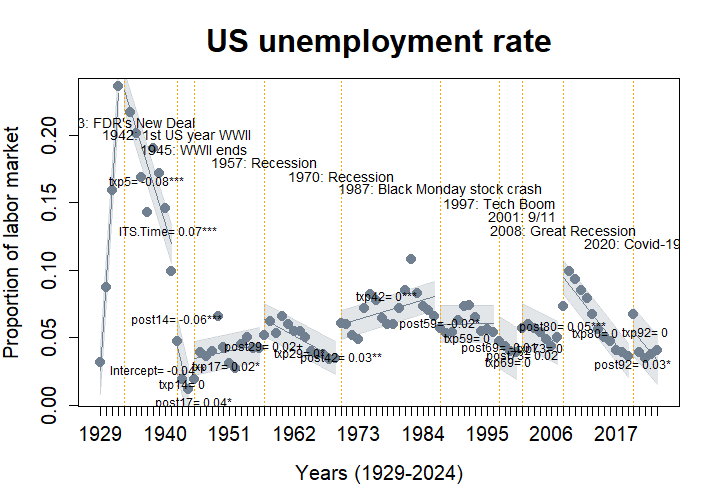
The most noticeable change was to add an option to allow as many interruptions as possible for Interrupted Time Series (ITS)
#Key interruption periods
key_time <- c(5, 14, 17, 29, 42, 59, 69, 73, 80,92)
im10 <- assess(formula=rate ~ ., data=unemployment, intervention = "usa",
int.time="year", its="one", interrupt= key_time, newdata=TRUE)plot(im10, "ITS", add.means = TRUE, coefs=TRUE, conf.int=TRUE,
adj.alpha= .2, lwd=1.75, col="slategray", tcol= "orange", main="US unemployment rate",
xlab="Years (1929-2024)", ylab= "Proportion of labor market", cex.main=2,
cex.axis = 1.25, cex.lab = 1.25, cex=2, cex.text= .75, pos.text=list("ITS.Time"=4,
"post42"=1,"txp42"=3,"txp92"=3), x.axis=unemployment$Year)
for(i in 1:length(key_time)) {
text(key_time[i], .22-(.01*i), cex=.85, labels =
paste0(unemployment[ key_time[i], "Year"], ": ", unemployment[ key_time[i], "event"]))
}
These and other changes included in version 1.2:
There are are options for a model summary and graphing. For example, below is a Posterior Predictive Check on how well our model fits the data. Estimating center and spread for hospital length of stay. A model with a gamma likelihood would fit better but this will do for demonstration purposes.
Other Bayesian options include multilevel summaries and graphs, posterior distribution summaries, model diagnostics, Gelman R^2 formula, and target setting.
blos1 <- Bayes(x=losmcmc)plot(x=blos1, y="post", parameter=list("sigmaOfY", "muOfY" ),math="divide",
bcol="cyan", HDItext=.3, main= "Coefficient of Variation")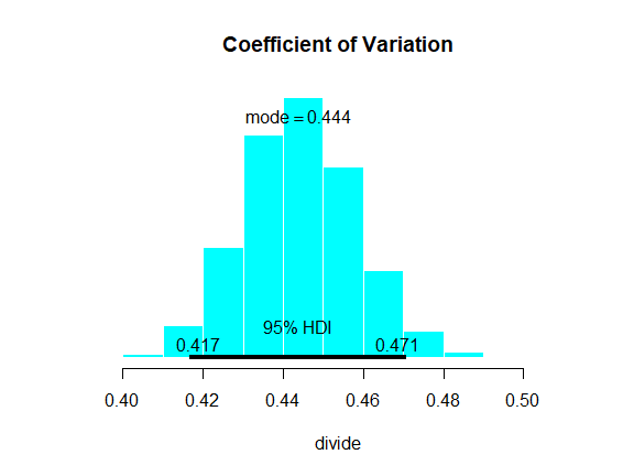
plot(x=blos1, y="check", type="n", data=hosprog, dv="los",
parameter=c("muOfY", "sigmaOfY"), breaks=30, cex.axis=1.3, lwd=3, xlab=NULL,
pline=20, vlim=c(-2, 20), xlim=c(-2, 20), add.legend="topright",
main="Length of Stay", cex.main=1.5, xpt=5, pcol="red", lcol="orange",
cex.legend=1, bcol="cyan")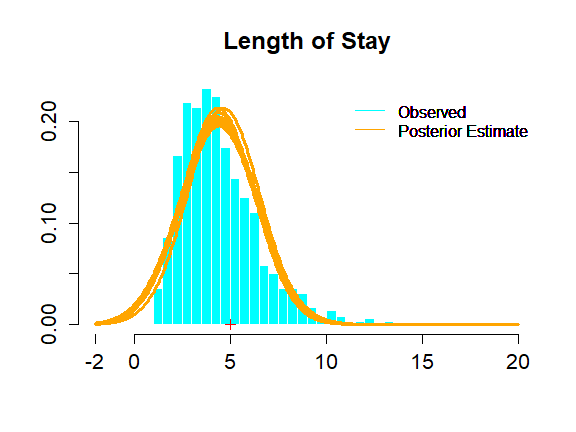
There are options for Shewhart X-bar charts, p-Charts, and u-Charts. This includes summary values and the charts. You can do a before-and-after comparison to see if there is a change too.
u-chart for infection rates with an intervention.
spc_u <- control(x="HAI", y="PatientDays", time="Month", data=infections,
type="u", n.equal=FALSE, intervention=22)
u-chart with trend lines, various graphing options, x.axis start at 2nd year and y.axis changed to show HAIs per 1,000 patient days.
plot(spc_u, main="u-Chart: HAI per 1,000 Patient Days Pre/Post Intervention",
col=c("green","dodgerblue"), trend=TRUE, trcol="red", x.axis=c((1:41+12)), round.c=1,
y.axis=seq(min(spc_u$HAI)*1000, max(spc_u$HAI)*1000, length.out=nrow(spc_u)),
xlab="Months (starting at year 2)", icol="gray", lwd=2, cex=2,
cex.axis=1.1, cex.main=1.25, cex.text=1.25)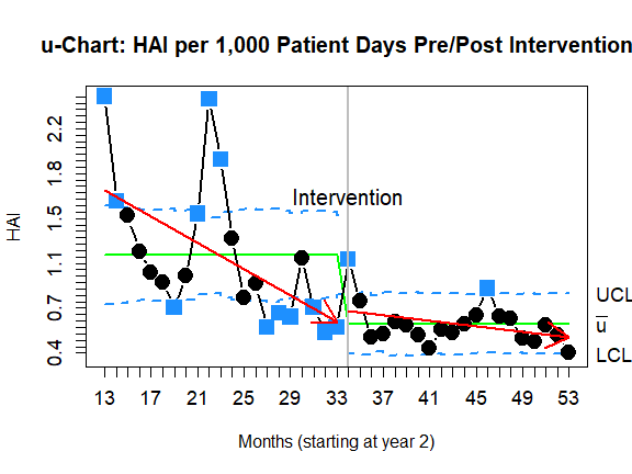
View decision curve analysis results like ‘net benefit’ at various thresholds of key interest at these percentiles: 0.01, 0.05, 0.10, 0.25, 0.50, 0.75, 0.90, 0.95, 0.99.
We’ll first start of with the model classification graph from a logistic regression model.
car_m1 <- assess(formula=vs ~ hp + am, data=mtcars, regression="logistic")
d1 <- decide(x=car_m1, threshold= -0.767)
print(d1$Model.Summary$Classification)
#>     Sensitivity       Specifity False.Positives False.Negatives   Accuracy.Rate
#>      0.92857143      0.83333333      0.16666667      0.07142857      0.87500000
#>      Error.Rate
#>      0.12500000
and next the graph.
plot(x=d1, y= "cl", cex.lab=.75, bcol=c("cyan", "magenta"), add.legend="topleft", cex.legend=1.5)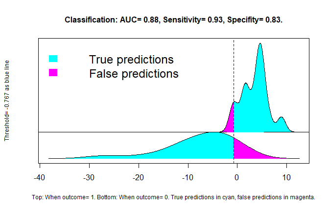
Now we’ll show ‘Net Benefit’
plot(x=d1, y= "nb", add.legend="topright", lwd=3, lcol=c("green", "slategray", "red"))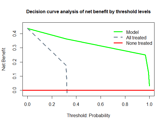
and then ‘Interventions Saved’
plot(x=d1, y= "is")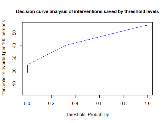
These and other changes included in version 1.4:
New additions
plot.Bayes variation analysis, multiple posterior predictive check lines
Partial prediction plots were added to show the trend line for continuous variables or 95% confidence intervals for categorical variables when the regression type is ‘ols’, ‘logistic’, ‘poisson’, or ‘coxph’. These trend lines control for the other predictors in the model.
Cox Proportional Hazards models from the survival package have been included for various options such as: partial prediction plots plot(), interpret(), importance(), review() and the various plot options. You would first need to convert it into an assess object like this: assess_obj <- assess(model = cox_model). And then you can use it with the functions listed above.
R2 and C-statistic/AUC were added to interpret() whenever possible for DID, ITS, and other regression models.
losvary Bayesian chains of hospital LOS added for plot.Bayes examples
compapt data of VA hospitals completed appointments for 1 month across locations
covshort data of hospital staffing critical shortage from US Dept. of Health on one day.
“decreasing” order argument when y=“multi” in plot.Bayes
Corrected errors
For the interrupted time-series interpretations, the phrases “one-group, multiple intervention period” and “two group, multiple time periods” are correctly stated with the relevant models.
For the interrupted time-series ITS effect summaries with itsEffect(), the lower and upper confidence limits were corrected. The point estimates, p-values, S.E., and t-statistic have always been correct.
The propensity score weights, “ipw”, “nipw”, and “att”, are now correct because the code was fixed.
The propensity score covariate and weights, “pscore”, “ipw”, “nipw”, and “att”, can be used in later regressions after the variables initial creation without causing the regression to get stopped with an error message.
In Bayes, the code was fixed so level 2 models can have their model summary created when y=“multi”.
The Bayesian data co2multi.rda was revised, with the above level 2 model correction.
The NHSN data now has the “logPredicted” variable as originally intended.
It was discovered that the coda and ham packages’ namespaces conflict. It is recommended to restart your R session after using coda and prior to using ham so that the ham functions will run as expected.
The Bayes vignette has typos fixed in the form of formatted bullets and “X.Lab” was correctly replaced with “xlab” in the multilevel plots.
This graph will be added in version 1.3 and it is a way to get a review of the coefficients, showing the direction of the effect with point estimates and 95% confidence intervals. This was inspired by Frank Harrell’s plot.summary in the rms package. Instead ham uses plot.review with the almost identical summary but adds some class information to help with plotting. This will work on assess regression objects for OLS linear, logistic, Poisson and models coming from Base R’s lm() and glm() as well as the survival package and possibly other glm() models. It can work with Cox Proportional Hazards from the survival package. And this will work with the differences-in-differences and interrupted time series models created with assess().
Take a look at the effect when hp is increased by 83.5
m02 <- assess(formula=mpg ~ wt+hp+am, data=mtcars, regression="ols")
# Using the assess function, notice 'm02$model' object below
print(review(m02$model), digits=4)
#> =================================================
#>                   Model Review
#> =================================================
#>    PointEst    Lower   Upper         P
#> wt -2.87900 -4.73200 -1.0250 0.0035740
#> hp -0.03748 -0.05715 -0.0178 0.0005464
#> am  2.08400 -0.73580  4.9030 0.1413000
#> =================================================
let’s see the impactful 83.5 hp increase in going from the 1st to 3rd quartiles
m02 <- assess(formula=mpg ~ wt+hp+am, data=mtcars, regression="ols")
plot(x=review(m02$model, increase=c(hp= 83.5)))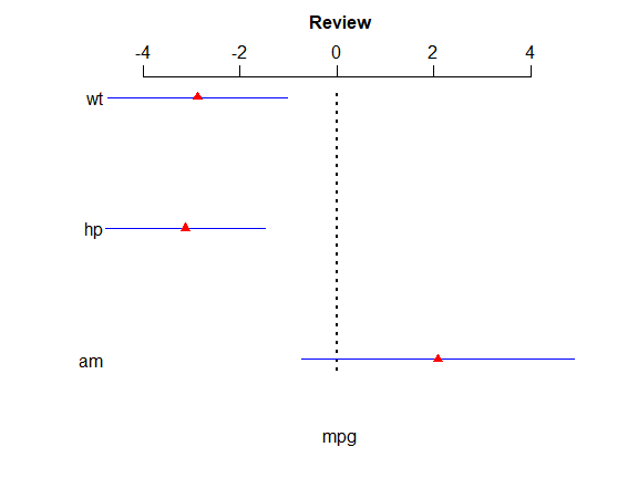
We now review the trend with a partial prediction plot. A partial prediction plot graphs the estimated trend of a continuous variable (or categorical) while holding all other variables constant at the other variables’ median value or reference level for categorical variables. This is for a range spanning the inner 95% of the target variable (i.e., Month’s trend line is graphed, holding other variables constant) and the predicted score is plotted against the range of Month values. Categorical variables have 95% confidence interval bars for each level. These calculations are performed in a manner similar to Professor Frank Harrell’s rms package.
We’ll review the partial prediction plot for the ‘count’, keeping in mind 100. These estimates are based on the median PatientDays and help to show the trend.
m04 <- assess(formula=HAI ~  Month+ offset(log(PatientDays)),
data=infections, regression="poisson")
plot(x=m04, y=c('Month', 'count'), col='skyblue', tgt=100, tgtcol='magenta', lwd=4)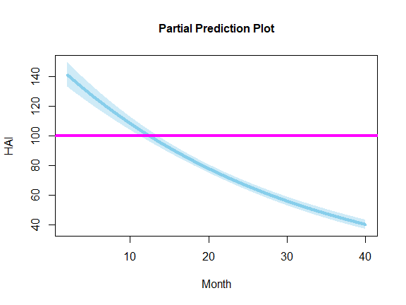
And a partial prediction plot option for categorical variables using 3 randomly generated categories with 95% confidence interval on effect.
infections$rand <- as.factor(sample(1:3, 41, replace = T))
m05 <- assess(HAI ~ Month + rand + offset(log(PatientDays)),
               data = infections, regression="poisson")
plot(x=m05, y=c('rand', 'count'), col='skyblue', tgt=75, tgtcol='orange', lwd=4, cex=2)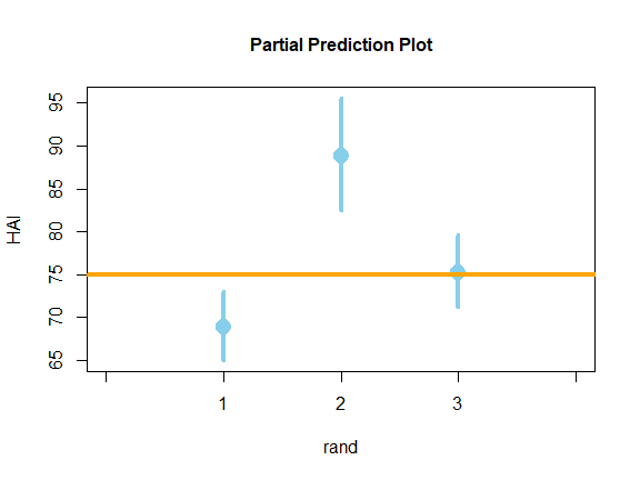
And now we’ll look at the partial predictions of the ‘Month’ variable for each level of a categorical variable by adding a 3rd element, y=c(‘Month’, ‘count’, ‘rand’). Because ‘count’ was specified and there is an offset, it returns estimates based on the median value of the offset variable. To do this for each level, you’ll always need 3 elements with the same type of info of the following, in the same order: y=c(my_continuous_variable, type_of_prediction, my_categorical_variable). Don’t forget to use the ‘add.legend’ and ‘col’ arguments to help highlight each level.
set.seed(1)
infections$rand <- as.factor(sample(1:3, 41, replace = T))
m05 <- assess(HAI ~ Month + rand + offset(log(PatientDays)),
               data = infections, regression="poisson")
plot(x=m05, y=c('Month', 'count', 'rand'), col=c('purple', 'gold','green'), add.legend= "topright", lwd=4, cex=2)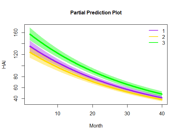
Here’s a new way to all diagnostics for the parameters with an interpretation
blos2 <- Bayes(losmcmc, y="Dx", parameter="muOfY")
interpret(blos2$Diagnostics, digits=5)
#> MCMC Diagnostics
#> ----------------
#> MCMC representativeness: The Gelman-Rubin statistic (shrink factor) measures
#> the ratio of within- and between-chain variance and is considered as having
#> a good range of 1.0 to 1.1 with a value of 1.0 indicating the chains are
#> fully converged and values above 1.1 suggesting the chains have not converged
#> yet. For MCMC representativeness graphs, please examine trace plots and
#> density plots found with plot(Bayes()).
#>
#> 1. According to the Gelman-Rubin Statistic (GRS) results, your MCMC first
#> reached the level below 1.1 by about step 100 in the chain.
#>
#> 2. The lowest GRS was 1. And 7 of the selected 7 steps between the first
#> and last steps in the MCMC had Gelman-Rubin statistics below 1.10.
#>
#> MCMC accuracy: 1) The autocorrelation factor (ACF) is a measure of chain step
#> concentration or clustering with values near 0 being ideal (indicating no
#> clustering) for each chain at various lags (interested in lags 1-20). In
#> other words, higher ACF indicates that it changes only gradually from step
#> to step. Values of 0 to 0.05 are essentially the same, very good, with
#> regards to the ESS formula (see below). 2) The effective sample size (ESS)
#> tells us the sample size of a completely non-correlated chain that yielded
#> the same info because we'd like a measure of how much independent info there
#> is in autocorrelated chains. An ESS of >= 10,000 is recommended. Note that
#> the ESS uses the ACF in its calculations with higher ACF leading to lower ESS.
#> 3) The Monte Carlo standard error (MCSE) = parameter Std. Dev. / sqrt(ESS)
#> with values on the parameter scale. If the MCSE is much smaller than the
#> parameter mean, this indicates a good MCSE.
#>
#> 1. Your average Autocorrelation Factor across chains is:
#> 0.00461, 0.00383, -0.00818, -0.01403, -0.00424 at the
#> 1st, 5th, 10th, 15th, and 20th lags.
#>
#> 2. Your Effective Sample Size is 20000 and is above the ideal target of 10,000
#> or more for sparse regions of the distributions (e.g., limits of 95% HDIs).
#>
#> 3. Your Monte Carlo Standard Error is 0.00052. Please compare this value with
#> the parameter's average to understand how large or small the MCSE is.
#>
#> MCMC efficiency: Please see Kruschke, 2015, to read more about efficiency such
#> as 1) using different samplers, 2) parallel R, 3) changing parametrizations of
#> the model, 4) and thinning chains (recording fewer steps).
#>
#> Background
#> ----------
#> We have 3 main quality goals when generating MCMC samples from our posterior
#> distribution: A) Chain values are representative of the posterior and there
#> is no excessive initial value influence, therefore our chains explore the full
#> posterior range. B) Chains are sufficiently large for accurate and stable
#> estimates (e.g., 95% HDI). C) Chains should be efficient in terms of
#> completion time and computing power.
#>
#> MCMC diagnostics help us with most of these goals and allows us to review:
#>
#> 1) Visual inspection of trace and density plots, see plot(Bayes()), and the
#> Gelman-Rubin statistic can suggest whether the burn-in period has been
#> suitably passed and
#> 2) suggests whether the chains are well-mixed and representative of the posterior.
#> 3) Remember these don't guarantee representativeness.
#> 4) ESS and MCSE suggest how stable and accurate the chains are.
#> 5) For stability in sparse regions (e.g., 95% HDI limits), ideally ESS >= 10,000.
#> 6) If you want accuracy in the dense regions of the distribution such as the mean,
#> a small MCSE may suggest the mean can be estimated very stably even with a low ESS.A possible healthcare target analysis with interpretations of results.
btarget1 <- Bayes(x=losmcmc, y="target", type="n", parameter=c("muOfY","sigmaOfY"),
newdata=TRUE, targets=list(p=c(.35,.4,.45, .5, .55),  y=c(3,4), e= list(a=c(.35,.4,.45), b=.5)))
interpret(btarget1$Target, digits=3)
#> Interpretations: Target
#> -----------------------
#> Based on the cumulative distribution function for P(X <= x),
#> the following probability is at or less than point x, with
#> 95% Highest Density Intervals [HDI Low, HDI High]:
#> The probability of x <= 3 is 0.232 [0.209, 0.259].
#> The probability of x <= 4 is 0.416 [0.385, 0.442].
#>
#> The estimated interval of the lowest and highest x values you
#> listed have this estimated area under the curve between them:
#> The AUC in the interval of 3 and 4 is 0.18 [0.171, 0.19].
#>
#> Based on the inverse cumulative distribution function for
#> P(X <= x) = p'th quantile, the following x is at this percentile,
#> with 95% Highest Density Intervals [HDI Low, HDI High]:
#> The 35th percentile of x is 3.69 [3.53, 3.82].
#> The 40th percentile of x is 3.92 [3.79, 4.08].
#> The 45th percentile of x is 4.18 [4.04, 4.33].
#> The 50th percentile of x is 4.43 [4.29, 4.58].
#> The 55th percentile of x is 4.67 [4.53, 4.82].
#>
#> The estimated interval of the lowest and highest percentile values you
#> listed have this estimated absolute difference in x between them:
#> The difference in the interval of 0.35 and 0.55 is 1.01 [0.953, 1.06].
#>
#> The estimated mean of the X values from the beta distribution
#> with 95% Highest Density Intervals [HDI Low, HDI High]:
#> NA
#>
#> Cohen's h effect sizes may help understand the difference in potential
#> targets, for the following absolute differences in proportions:
#> The effect size of 0.5 minus 0.35 is 0.305, a small effect.
#> The effect size of 0.5 minus 0.4 is 0.201, a small effect.
#> The effect size of 0.5 minus 0.45 is 0.1, a less than small effect.Two types of variation can be reviewed with Bayesian analysis: 1) Conduct a Bayesian differences-in-differences analysis in which the DID is calculated for the variation parameter of the model (e.g., standard deviation) and graph the posterior predictive checks at pre-test over the observed post-test data to view the change or 2) compare and contrast lines from multiple posterior predictive checks of parameters to see the difference in estimated distributions.
Here is an example of the 1st option of the variation DID but this same plot code works for the 2nd option.
Below, we have code to do a variation analysis of a model with a log-normal distribution for length of stay (LOS). The losvary object requires we modify the hosprog data by adding the predictor variable for ‘Post.Int’.
# These make 4 levels for the intervention program * pre/post period
#pre/post indicator
hosprog$prepost <- ifelse(hosprog$month >= 5, 1, 0)
#Control group at pre-test
hosprog$Post.Int <- 1
#Control group at post-test
hosprog[, "Post.Int"][hosprog$program == 0 & hosprog$prepost == 1 ] <- 2
#Intervention group at pre-test
hosprog[, "Post.Int"][hosprog$program == 1 & hosprog$prepost == 0 ] <- 3
#Intervention group at post-test
hosprog[, "Post.Int"][hosprog$program == 1 & hosprog$prepost == 1 ] <- 4
Now we can create the ham object.
bvlos <- Bayes(x=losvary, newdata=TRUE)
#key parameters for post check
parls <- list(c("muOfLogY[1]", "sigmaOfLogY[1]"),
              c("muOfLogY[2]", "sigmaOfLogY[2]"),
              c("muOfLogY[3]", "sigmaOfLogY[3]"),
              c("muOfLogY[4]", "sigmaOfLogY[4]"))
We’ll first look at the DID for variation. We see the amount is about a 1 day reduction in standard deviation for the treatment group. In other words, the control group increased standard deviation in the post-intervention period by 1/2 a day while the treatment group decreased by 1/2 a day. The estimates aren’t found in the losvary object but it comes out to about equivalent to this calculation: (1.5 - 2.1) - (2.0 - 1.6) = -1.
plot(x=bvlos, y="post", parameter="B3DIDSig", bcol="green", compare=0,
     HDItext=.3, cex=2, main= "B3DIDSig")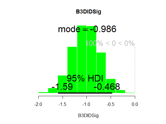
Let’s take a look at the various posterior predictive checks, this will give us insight in how the control and treatment groups vary by pre/post intervention periods. Note that the grey observed data bars are all data and only 1 single line for each parameter is used for clarity in the lower zoomed in section.
plot(x=bvlos, y="vary", type="ln", dv="los", breaks=75, pline=3, lwd=1, vlim=c(0, 15),
     data=hosprog, lcol= c("pink","red", "cyan", "blue"), xlim=c(0.5, 15), ylim=c(0, .35), parameter=parls, main="LOS and posterior pred checks", cex.main=2, cex.legend=1.5, cex.label=1.5,
     cex.axis=1.5, add.legend="topright", legend=c("Observed Data", "CTL Pre Est.", "CTL Post Est.", "Treat Pre Est.", "Treat Post Est."))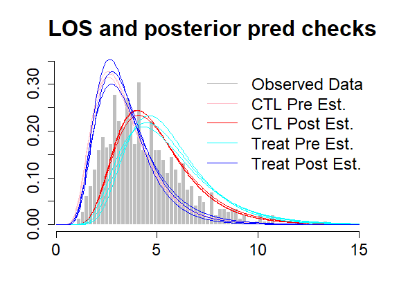
The lighter colors represent the pre-intervention time. For example, the pink line shows lower LOS for the control group which is similar to the blue line for the treatment group’s post-intervention period. In other words, things got better for the treatment group’s LOS while things got worse for the control group.
Now we zoom in on the tails that represent the high lengths of stay.
plot(x=bvlos, y="vary", type="ln", dv="los", breaks=75, pline=1, lwd=5, vlim=c(0, 15),
     data=hosprog, lcol= c("pink","red", "cyan", "blue"), xlim=c(10, 15), ylim=c(0, .03), parameter=parls, main="LOS Zoomed In", cex.main=2, cex.legend=1.5, cex.label=1.5,
     cex.axis=1.5, add.legend="topright", legend=c("Observed Data", "CTL Pre Est.", "CTL Post Est.", "Treat Pre Est.", "Treat Post Est."))