The hydraulics R package solves basic pipe hydraulics for both pressure and gravity flow conditions, and open-channel hydraulics for trapezoidal channels, including triangular and rectangular. Pressure pipe solutions include functions to 1) describe properties of water, 2) solve the Darcy-Weisbach equation for friction loss through pipes, and 3) plot a Moody diagram. There are also functions for matching a pump characteristic curve to a system curve, and solving for flows in a pipe network using the Hardy-Cross method. Partially-filled pipe and other open-channel flow solutions are solved with the Manning equation. The format of functions and pressure pipe solutions are designed to be compatible with the iemisc package, and the open channel hydraulics solutions are modifications of code in that package.
![]()
#Install the stable CRAN version of this package
install.packages("hydraulics")
#Install the development version of this package
if (!requireNamespace("remotes", quietly = TRUE)) install.packages("remotes")
remotes::install_github("EdM44/hydraulics")library(hydraulics)D <- 20/12 #20 inch converted to ft
L <- 10560 #ft
Q <- 4 #ft3/s
T <- 60 #F
ks <- 0.0005 #ft
#Optionally, use utility functions to find the Reynolds Number and friction factor, f:
reynolds_number(V = velocity(D, Q), D = D, nu = kvisc(T = T, units = "Eng"))
#> [1] 248624.7
colebrook(ks = ks, V = velocity(D, Q), D = D, nu = kvisc(T = T, units = "Eng"))
#> [1] 0.0173031
#Solve directly for the missing value of friction loss
ans1 <- darcyweisbach(Q = Q,D = D, L = L, ks = ks, nu = kvisc(T=T, units="Eng"), units = c("Eng"))
#> hf missing: solving a Type 1 problem
cat(sprintf("Reynolds no: %.0f\nFriction Fact: %.4f\nHead Loss: %.2f ft\n", ans1$Re, ans1$f, ans1$hf))
#> Reynolds no: 248625
#> Friction Fact: 0.0173
#> Head Loss: 5.72 ftD <- .5 #m
L <- 10 #m
hf <- 0.006*L #m
T <- 20 #C
ks <- 0.000046 #m
ans2 <- darcyweisbach(D = D, hf = hf, L = L, ks = ks, nu = kvisc(T=T, units='SI'), units = c('SI'))
#> Q missing: solving a Type 2 problem
cat(sprintf("Reynolds no: %.0f\nFriction Fact: %.4f\nFlow: %.2f m3/s\n", ans2$Re, ans2$f, ans2$Q))
#> Reynolds no: 1010337
#> Friction Fact: 0.0133
#> Flow: 0.41 m3/sQ <- 37.5 #flow in ft^3/s
L <- 8000 #pipe length in ft
hf <- 215 #head loss due to friction, in ft
T <- 68 #water temperature, F
ks <- 0.0008 #pipe roughness, ft
ans3 <- darcyweisbach(Q = Q, hf = hf, L = L, ks = ks, nu = kvisc(T=T, units='Eng'), units = c('Eng'))
#> D missing: solving a Type 3 problem
cat(sprintf("Reynolds no: %.0f\nFriction Fact: %.4f\nDiameter: %.2f ft\n", ans3$Re, ans3$f, ans3$D))
#> Reynolds no: 2336974
#> Friction Fact: 0.0164
#> Diameter: 1.85 ftD <- 1.85 #diameter in ft
Q <- 37.5 #flow in ft^3/s
L <- 8000 #pipe length in ft
hf <- 215 #head loss due to friction, in ft
T <- 68 #water temperature, F
ans4 <- darcyweisbach(Q = Q, D = D, hf = hf, L = L, nu = kvisc(T=T, units='Eng'), units = c('Eng'))
#> ks missing: solving for missing roughness height
knitr::kable(setNames(as.data.frame(unlist(ans4)),c('value')), format = "html", padding=0)| value | |
|---|---|
| Q | 3.750000e+01 |
| V | 1.395076e+01 |
| L | 8.000000e+03 |
| D | 1.850000e+00 |
| hf | 2.150000e+02 |
| f | 1.649880e-02 |
| ks | 8.176000e-04 |
| Re | 2.335866e+06 |
nu = kvisc(T = 55, units = 'Eng')
cat(sprintf("Kinematic viscosity: %.3e ft2/s\n", nu))
#> Kinematic viscosity: 1.318e-05 ft2/snu = kvisc(units = 'Eng')
#>
#> Temperature not given.
#> Assuming T = 68 F
cat(sprintf("Kinematic viscosity: %.3e ft2/s\n", nu))
#> Kinematic viscosity: 1.105e-05 ft2/srho = dens(T = 25, units = 'SI')
cat(sprintf("Water density: %.3f kg/m3\n", rho))
#> Water density: 997.075 kg/m3moody(Re = c(ans1$Re, ans2$Re, ans3$Re), f = c(ans1$f, ans2$f, ans3$f))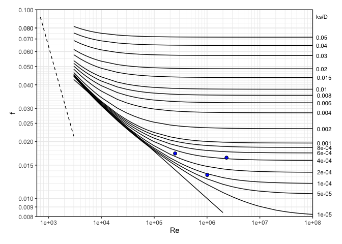
oc1 <- manningc(d = 0.6, n = 0.013, Sf = 1./400., y = 0.24, units = "SI")
cat(sprintf("Flow rate, Q: %.2f m3/s\nFull pipe flow rate, Qf: %.2f\n", oc1$Q, oc1$Qf))
#> Flow rate, Q: 0.10 m3/s
#> Full pipe flow rate, Qf: 0.31oc2 <- manningc(Q = 83.5, n = 0.015, Sf = 0.0002, y_d = 0.9, units = "Eng")
cat(sprintf("Required diameter: %.2f ft\nFlow depth: %.2f\n", oc2$d, oc2$y))
#> Required diameter: 7.00 ft
#> Flow depth: 6.30xc_circle( y = oc2$y ,d = oc2$d, units = "Eng" )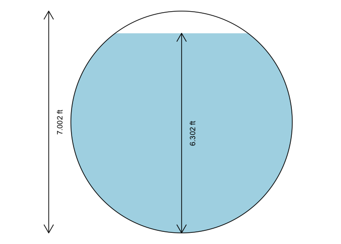
oc3 <- manningt(Q = 360., n = 0.015, m = 1, b = 20.0, y = 3.0, units = "Eng")
cat(sprintf("Slope: %.5f ft\nCritical depth: %.2f\n", oc3$Sf, oc3$yc))
#> Slope: 0.00088 ft
#> Critical depth: 2.08spec_energy_trap( Q = oc3$Q, b = oc3$b, m = oc3$m, scale = 4, units = "Eng" )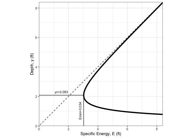
xc_trap( y = oc3$y, b = oc3$b, m = oc3$m, units = "Eng" )
#> Warning in ggplot2::geom_segment(data = seg1, ggplot2::aes(x = 0, xend = -0.1 * : All aesthetics have length 1, but the data has 2 rows.
#> ℹ Please consider using `annotate()` or provide this layer with data containing
#>   a single row.
#> Warning in ggplot2::geom_segment(data = seg1, ggplot2::aes(x = B, xend = B + : All aesthetics have length 1, but the data has 2 rows.
#> ℹ Please consider using `annotate()` or provide this layer with data containing
#>   a single row.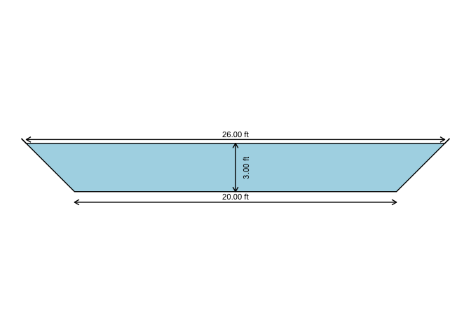
For other functions related to pump characteristic curves and operating point determination, and pipe network solutions, refer to the hydraulics vignette.