Implementation of Warnes & Raftery’s MCGibbsit
run-length diagnostic for a set of (not-necessarily independent) Markov
Chain Monte Carlo (MCMC) samplers.
It combines the estimate error-bounding approach of the Raftery and
Lewis MCMC run length diagnostic (gibbsit) with the between
verses within chain approach of the Gelman and Rubin MCMC convergence
diagnostic.
Install the most recent release from CRAN:
install.packages("mcgibbsit")Or the current development version from github:
if(!require("remotes"))
  install.packages("remotes")

remotes::install_github('r-gregmisc/mcgibbsit')library(mcgibbsit)
#> Loading required package: coda
set.seed(42) # for reproducibility
tmpdir <- tempdir()The mcgibbsit package provides an implementation of
Warnes & Raftery’s MCGibbsit run-length diagnostic for a set of
(not-necessarily independent) MCMC samplers. It combines the estimate
error-bounding approach of Raftery and Lewis with the between chain
variance verses within chain variance approach of Gelman and Rubin.
mcgibbsit computes the minimum run length \(N_{min}\), required burn in \(M\), total run length \(N\), run length inflation due to
auto-correlation, \(I\), and
the run length inflation due to between-chain correlation,
\(R\) for a set of exchangeable MCMC
simulations which need not be independent.
The normal usage is to perform an initial MCMC run of some
pre-determined length (e.g. 300 iterations) for each of a set of \(k\) (e.g. 20) MCMC samplers. The output
from these samplers is then read in to create an mcmc.list
object and mcgibbsit is run specifying the desired accuracy
of estimation for quantiles of interest. This will return the minimum
number of iterations to achieve the specified error bound. The set of
MCMC samplers is now run so that the total number of iterations exceeds
this minimum, and mcgibbsit is again called. This should
continue until the number of iterations already complete is less than
the minimum number computed by mcgibbsit.
If the initial number of iterations in data is too small
to perform the calculations, an error message is printed indicating the
minimum pilot run length.
This basic example constructs a dummy set of files from an
imaginary MCMC sampler and shows the results of running
mcgibbsit with the default settings.
# Define a function to generate the output of our imaginary MCMC sampler
gen_samples <- function(run_id, nsamples=200)
{
  x <- matrix(nrow = nsamples+1, ncol=4)
  colnames(x) <- c("alpha","beta","gamma", "nu")

  x[,"alpha"] <- exp(rnorm (nsamples+1, mean=0.025, sd=0.025))
  x[,"beta"]  <- rnorm (nsamples+1, mean=53,    sd=14)
  x[,"gamma"] <- rbinom(nsamples+1, 20,         p=0.15) + 1
  x[,"nu"]    <- rnorm (nsamples+1, mean=x[,"alpha"] * x[,"beta"], sd=1/x[,"gamma"])
#'
  # induce serial correlation of 0.25
  x <- 0.75 * x[2:(nsamples+1),] + 0.25 * x[1:nsamples,]

  # induce ~50% acceptance rate
  accept <- runif(nsamples) > 0.50
  for(i in 2:nsamples)
    if(!accept[i]) x[i,] <- x[i-1,]

  write.table(
    x,
    file = file.path(
      tmpdir,
      paste("mcmc", run_id, "csv", sep=".")
      ),
    sep = ",",
    row.names = FALSE
  )
}
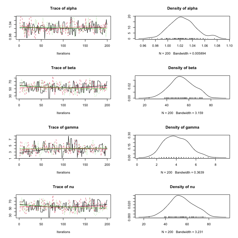
First, we’ll generate and load only a 3 runs of length 200:
# Generate and load 3 runs
for(i in 1:3)
  gen_samples(i, 200)

mcmc.3 <- read.mcmc(
  3,
  file.path(tmpdir, "mcmc.#.csv"),
  sep=",",
  col.names=c("alpha","beta","gamma", "nu")
  )
# Trace and Density Plots
plot(mcmc.3)
Now run mcgibbsit to determine the necessary total
number of MCMC samples to to provide accurate 95% posterior confidence
region estimates for all four of the parameters:
# And check the necessary run length
mcg.3 <- mcgibbsit(mcmc.3)
print(mcg.3)
#>                   Multi-Chain Gibbsit
#>                   -------------------
#>
#> Call             = mcgibbsit(data = mcmc.3)
#>
#> Number of Chains = 3
#> Per-Chain Length = 200
#> Total Length     = 600
#>
#> Quantile (q)     = 0.025
#> Accuracy (r)     = +/- 0.0125
#> Probability (s)  = 0.95
#>
#>
#>       Burn-in  Estimation Total Lower bound  Auto-Corr. Between-Chain
#>       (M)      (N)        (M+N) (Nmin)       factor (I) Corr. factor (R)
#>
#> alpha 24       1301       1325  600          2.28       0.955
#> beta  33       1830       1863  600          3.22       0.951
#> gamma 27       1932       1959  600          2.74       1.180
#> nu    33       1849       1882  600          3.22       0.961
#>       -----    -----      ----- -----        -----      -----
#>       33       1932       1959  600
#>
#> NOTE: The values for M, N, and Total are combined numbers of iterations
#>       based on using 3 chains.
The results from mcgibbsit indicate that the required
number of samples is 1,959, which is less than we’ve generated so
far.
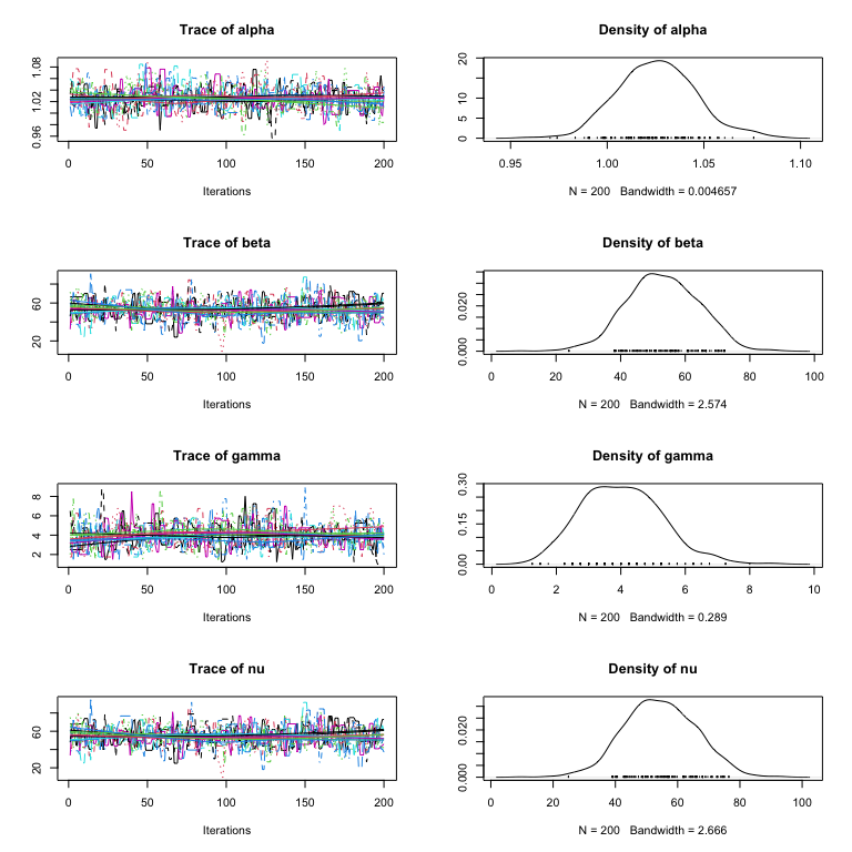
Lets generate 7 more runs, each of length 200, for a total of 2,000 samples:
# Generate and load 7 more runs
for(i in 3 + (1:7))
  gen_samples(i, 200)

mcmc.10 <- read.mcmc(
  10,
  file.path(tmpdir, "mcmc.#.csv"),
  sep=",",
  col.names=c("alpha","beta","gamma", "nu")
  )
# Trace and Density Plots
plot(mcmc.10)
Now run mcgibbsit to determine the necessary number of
MCMC samples:
# And check the necessary run length
mcg.10 <- mcgibbsit(mcmc.10)
print(mcg.10)
#>                   Multi-Chain Gibbsit
#>                   -------------------
#>
#> Call             = mcgibbsit(data = mcmc.10)
#>
#> Number of Chains = 10
#> Per-Chain Length = 200
#> Total Length     = 2000
#>
#> Quantile (q)     = 0.025
#> Accuracy (r)     = +/- 0.0125
#> Probability (s)  = 0.95
#>
#>
#>       Burn-in  Estimation Total Lower bound  Auto-Corr. Between-Chain
#>       (M)      (N)        (M+N) (Nmin)       factor (I) Corr. factor (R)
#>
#> alpha 90       1534       1624  600          2.76       0.933
#> beta  110      1743       1853  600          3.11       0.940
#> gamma 90       1820       1910  600          3.19       0.955
#> nu    100      1569       1669  600          2.79       0.942
#>       -----    -----      ----- -----        -----      -----
#>       110      1820       1910  600
#>
#> NOTE: The values for M, N, and Total are combined numbers of iterations
#>       based on using 10 chains.
mcgibbsit now estimates that a total of required number
of samples is 1,910 (this is slightly fewer than before because the the
larger number of samples allowed more accurate estimates of the
variances and correlations). Since we we have already generated 2,000
samples, we do not need to perform any additional runs.
We can now calculate the posterior confidence regions for each of the parameters.
summary(mcmc.10)
#>
#> Iterations = 1:200
#> Thinning interval = 1
#> Number of chains = 10
#> Sample size per chain = 200
#>
#> 1. Empirical mean and standard deviation for each variable,
#>    plus standard error of the mean:
#>
#>         Mean       SD  Naive SE Time-series SE
#> alpha  1.026  0.02033 0.0004546       0.000787
#> beta  53.012 11.10534 0.2483230       0.433342
#> gamma  4.024  1.24685 0.0278804       0.046729
#> nu    54.391 11.50530 0.2572663       0.438652
#>
#> 2. Quantiles for each variable:
#>
#>          2.5%    25%    50%    75% 97.5%
#> alpha  0.9892  1.012  1.025  1.039  1.07
#> beta  31.1137 45.587 52.633 60.664 73.74
#> gamma  1.7500  3.000  4.000  4.750  6.75
#> nu    32.3646 46.484 54.455 61.896 76.44