![]()
![]()
![]()

![]()
![]()
metrica is a compilation of more than 80 functions
designed to quantitatively and visually evaluate the prediction
performance of regression (continuous variables) and classification
(categorical variables) point-forecast models (e.g. APSIM, DSSAT, DNDC,
Supervised Machine Learning). metrica offers a toolbox with
a wide spectrum of goodness of fit, error metrics, indices, and
coefficients accounting for different aspects of the agreement between
predicted and observed values, plus some basic visualization functions
to assess models performance (e.g. confusion matrix, scatter with
regression line; Bland-Altman plot) provided in customizable format
(ggplot).
For supervised models, always keep in mind the concept of
“cross-validation” since predicted values should ideally come from
out-of-bag samples (unseen by training sets) to avoid overestimation of
the prediction performance.
Check the Documentation at https://adriancorrendo.github.io/metrica/
Vignettes
1.
List of metrics for Regression
2.
List of metrics for Classification
3.
A regression case (numerical variables)
4.
A classification case (categorical variables)
For regression models, it includes 4 plotting functions (scatter,
tiles, density, & Bland-Altman plots), and 48 prediction performance
scores including error metrics (MBE, MAE, RAE, RMAE, MAPE, SMAPE, MSE,
RMSE, RRMSE, RSR, PBE, iqRMSE), error decomposition (MLA, MLP, PLA, PLP,
PAB, PPB, SB, SDSD, LCS, Ub, Uc, Ue), model efficiency (NSE, E1, Erel,
KGE), indices of agreement (d, d1, d1r, RAC, AC, lambda), goodness of
fit (r, R2, RSS, TSS, RSE), adjusted correlation coefficients (CCC, Xa,
distance correlation-dcorr-, maximal information coefficient -MIC-),
variability (uSD, var_u), and symmetric regression coefficients (B0_sma,
B1_sma). Specifically for time-series predictions, metrica
also includes the Mean Absolute Scaled Error (MASE).
For classification (binomial and multinomial) tasks, it includes a
function to visualize the confusion matrix using ggplot2, and 27
functions of prediction scores including: accuracy, error rate,
precision (predictive positive value -ppv-), recall (or true positive
rate-TPR-), specificity (or true negative rate-TNR-, or selectivity),
balanced accuracy (balacc), F-score (fscore), adjusted F-score (agf),
G-mean (gmean), Bookmaker Informedness (bmi, a.k.a. Youden’s J-index
-jindex-), Markedness (deltaP, or mk), Matthews Correlation Coefficient
(mcc, a.k.a. phi-coefficient), Cohen’s Kappa (khat), negative predictive
value (npv), positive and negative likelihood ratios (posLr, negLr),
diagnostic odds ratio (dor), prevalence (preval), prevalence threshold
(preval_t), critical success index (csi, a.k.a. threat score or Jaccard
Index -jaccardindex-), false positive rate (FPR), false negative rate
(FNR), false detection rate (FDR), false omission rate (FOR), and area
under the ROC curve (AUC_roc).
metrica also offers a function () that allows users to
run all prediction performance scores at once. The user just needs to
specify the type of model (“regression” or “classification”).
For more details visit the vignettes https://adriancorrendo.github.io/metrica/.
There are two basic arguments common to all metrica
functions: (i) obs(Oi; observed, a.k.a. actual, measured,
truth, target, label), and (ii) pred (Pi; predicted, a.k.a.
simulated, fitted, modeled, estimate) values.
Optional arguments include data that allows to call an
existing data frame containing both observed and predicted vectors, and
tidy, which controls the type of output as a list (tidy =
FALSE) or as a data.frame (tidy = TRUE).
For regression, some specific functions for regression also require
to define the axis orientation. For example, the slope of
the symmetric linear regression describing the bivariate scatter (SMA).
For binary classification (two classes), functions also require to
check the pos_level arg., which indicates the alphanumeric
order of the “positive level”. Normally, the most common binary
denominations are c(0,1), c(“Negative”, “Positive”), c(“FALSE”, “TRUE”),
so the default pos_level = 2 (1, “Positive”, “TRUE”). However, other
cases are also possible, such as c(“Crop”, “NoCrop”) for which the user
needs to specify pos_level = 1.
For multiclass classification tasks, some functions present the
atom arg. (logical TRUE / FALSE), which controls the output
to be an overall average estimate across all classes, or a class-wise
estimate. For example, user might be interested in obtaining estimates
of precision and recall for each possible class of the prediction.
You can install the CRAN version of metrica with:
install.packages("metrica")You can install the development version from GitHub with:
# install.packages("devtools")
devtools::install_github("adriancorrendo/metrica")The metrica package comes with four example datasets of
continuous variables (regression) from the APSIM software:
wheat. 137 data-points of wheat grain N (grams per
squared meter) barley. 69 data-points of barley grain number (x1000
grains per squared meter) sorghum. 36 data-points of sorghum grain number (x1000
grains per squared meter) chickpea. 39 data-points of chickpea aboveground dry
mass (kg per hectare) These data correspond to the latest, up-to-date, documentation and
validation of version number 2020.03.27.4956. Data available at: https://doi.org/10.7910/DVN/EJS4M0. Further details can
be found at the official APSIM Next Generation website: https://APSIMnextgeneration.netlify.app/modeldocumentation
In addition, metrica also provides two native examples
for categorical variables (classification):
land_cover is a binary dataset of land cover using
satellite images obtained in 2022 over a small region in Kansas (USA).
Values equal to 1 are associated to vegetation, and values equal to 0
represent other type of land cover. Observed values come from human
visualization, while predicted values were obtained with a Random Forest
classifier.
maize_phenology is a data set of maize/corn (Zea
mays L.) phenology (crop development stage) collected in Kansas
(USA) during 2018. The data includes 16 different phenology stages.
Observed values were obtained via human visualization, while predicted
values were obtained with a Random Forest classifier.
Any of the above-mentioned data sets can be called with
metrica::name_of_dataset, for example:
metrica::wheat
metrica::land_coverlibrary(metrica)
library(dplyr)
library(purrr)
library(ggplot2)
library(tidyr)This is a basic example which shows you the core regression and
classification functions of metrica:
# 1. A. Create a random dataset
# Set seed for reproducibility
set.seed(1)
# Create a random vector (X) with 100 values
X <- rnorm(n = 100, mean = 0, sd = 10)
# Create a second vector (Y) with 100 values by adding error with respect
# to the first vector (X).
Y <- X + rnorm(n=100, mean = 0, sd = 3)
# Merge vectors in a data frame, rename them as synonyms of observed (measured) and predicted (simulated)
example.data <- data.frame(measured = X, simulated = Y)

# 1. B. Or call native example datasets

example.data <- barley %>%  # or 'wheat', 'sorghum', or 'chickpea'
# 1.b. create columns as synonyms of observed (measured) and predicted (simulated)
                mutate(measured = obs, simulated = pred)
barley.scat.plot <-
  metrica::scatter_plot(data = example.data,
                        obs = measured,
                        pred = simulated,
                        orientation = "PO",
                        print_eq = TRUE,
                        position_eq = c(x=24, y =8),
                        # Optional arguments to customize the plot
                        shape_type = 21,
                        shape_color = "grey15",
                        shape_fill = "steelblue",
                        shape_size = 3,
                        regline_type = "F1",
                        regline_color = "#9e0059",
                        regline_size = 2)+
  # Customize axis breaks
  scale_y_continuous(breaks = seq(0,30, by = 5))+
  scale_x_continuous(breaks = seq(0,30, by = 5))

barley.scat.plot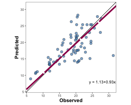
# Alternative using vectors instead of dataframe
#metrica::scatter_plot(obs = example.data$obs, pred = example.data$pred)barley.tiles.plot <-
tiles_plot(data = example.data,
obs = measured,
pred = simulated,
bins = 10,
orientation = "PO",
colors = c(low = "pink", high = "steelblue"))
barley.tiles.plot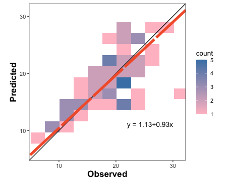
barley.density.plot <-
metrica::density_plot(data = example.data,
                      obs = measured, pred = simulated,
                      n = 5,
                      orientation = "PO",
           colors = c(low = "white", high = "steelblue") )+
  theme(legend.position = "none")

barley.density.plot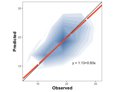
barley.ba.plot <- metrica::bland_altman_plot(data = example.data,
                                             obs = measured, pred = simulated)

barley.ba.plot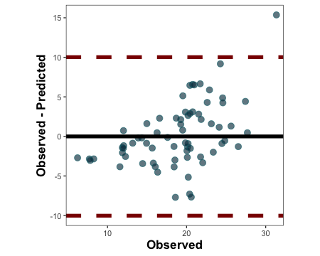
# a. Estimate coefficient of determination (R2)

metrica::R2(data = example.data, obs = measured, pred = simulated)
#> $R2
#> [1] 0.4512998

# b. Estimate root mean squared error (RMSE)
metrica::RMSE(data = example.data, obs = measured, pred = simulated)
#> $RMSE
#> [1] 3.986028

# c. Estimate mean bias error (MBE)
metrica::MBE(data = example.data, obs = measured, pred = simulated)
#> $MBE
#> [1] 0.207378

# c. Estimate index of agreement (d)
metrica::d(data = example.data, obs = measured, pred = simulated)
#> $d
#> [1] 0.8191397

# e. Estimate SMA regression intercept (B0)
metrica::B0_sma(data = example.data, obs = measured, pred = simulated, tidy = TRUE)
#>         B0
#> 1 1.128274

# f. Estimate SMA regression slope (B1)
metrica::B1_sma(data = example.data, obs = measured, pred = simulated)
#> $B1
#> [1] 0.9288715
metrics.sum <- metrics_summary(data = example.data,
                               obs = measured, pred = simulated,
                               type = "regression")
# Print first 15
head(metrics.sum, n = 15)
#>    Metric      Score
#> 1      B0  1.1282743
#> 2      B1  0.9288715
#> 3       r  0.6717885
#> 4      R2  0.4512998
#> 5      Xa  0.9963915
#> 6     CCC  0.6693644
#> 7     MAE  3.0595501
#> 8    RMAE  0.1629325
#> 9    MAPE 16.8112673
#> 10  SMAPE 16.7848032
#> 11    RAE  0.7639151
#> 12    RSE  0.6164605
#> 13    MBE  0.2073780
#> 14    PBE  1.1043657
#> 15    PAB  0.2706729

# Optional wrangling (WIDE)
metrics.sum.wide <- metrics.sum %>%
  tidyr::pivot_wider(tidyr::everything(),
                      names_from = "Metric",
                      values_from = "Score")

metrics.sum.wide
#> # A tibble: 1 × 45
#>      B0    B1     r    R2    Xa   CCC   MAE  RMAE  MAPE SMAPE   RAE   RSE   MBE
#>   <dbl> <dbl> <dbl> <dbl> <dbl> <dbl> <dbl> <dbl> <dbl> <dbl> <dbl> <dbl> <dbl>
#> 1  1.13 0.929 0.672 0.451 0.996 0.669  3.06 0.163  16.8  16.8 0.764 0.616 0.207
#> # ℹ 32 more variables: PBE <dbl>, PAB <dbl>, PPB <dbl>, MSE <dbl>, RMSE <dbl>,
#> #   RRMSE <dbl>, RSR <dbl>, iqRMSE <dbl>, MLA <dbl>, MLP <dbl>, RMLA <dbl>,
#> #   RMLP <dbl>, SB <dbl>, SDSD <dbl>, LCS <dbl>, PLA <dbl>, PLP <dbl>,
#> #   Ue <dbl>, Uc <dbl>, Ub <dbl>, NSE <dbl>, E1 <dbl>, Erel <dbl>, KGE <dbl>,
#> #   d <dbl>, d1 <dbl>, d1r <dbl>, RAC <dbl>, AC <dbl>, lambda <dbl>,
#> # dcorr <dbl>, MIC <dbl># a. Create nested df with the native examples
nested.examples <- bind_rows(list(wheat = metrica::wheat,
barley = metrica::barley,
sorghum = metrica::sorghum,
chickpea = metrica::chickpea),
.id = "id") %>%
dplyr::group_by(id) %>% tidyr::nest() %>% dplyr::ungroup()
head(nested.examples %>% group_by(id) %>% dplyr::slice_head(n=2))
#> # A tibble: 4 × 2
#> # Groups: id [4]
#> id data
#> <chr> <list>
#> 1 barley <tibble [69 × 2]>
#> 2 chickpea <tibble [39 × 2]>
#> 3 sorghum <tibble [36 × 2]>
#> 4 wheat <tibble [137 × 2]>
# b. Run
multiple.sum <- nested.examples %>%
# Store metrics in new.column "performance"
mutate(performance = map(
data, ~metrica::metrics_summary(data=., obs = obs, pred = pred,
type = "regression")))
head(multiple.sum)
#> # A tibble: 4 × 3
#> id data performance
#> <chr> <list> <list>
#> 1 wheat <tibble [137 × 2]> <df [45 × 2]>
#> 2 barley <tibble [69 × 2]> <df [45 × 2]>
#> 3 sorghum <tibble [36 × 2]> <df [45 × 2]>
#> 4 chickpea <tibble [39 × 2]> <df [45 × 2]>non_nested_summary <- nested.examples %>% unnest(cols = "data") %>%
group_by(id) %>%
summarise(metrics_summary(obs = obs, pred = pred, type = "regression")) %>%
dplyr::arrange(Metric)
head(non_nested_summary)
#> # A tibble: 6 × 3
#> # Groups: id [4]
#> id Metric Score
#> <chr> <chr> <dbl>
#> 1 barley AC 0.253
#> 2 chickpea AC 0.434
#> 3 sorghum AC 0.0889
#> 4 wheat AC 0.842
#> 5 barley B0 1.13
#> 6 chickpea B0 -99.0df <- metrica::wheat
# Create list of selected metrics
selected.metrics <- c("MAE","RMSE", "RRMSE", "R2", "NSE", "KGE", "PLA", "PLP")
df <- metrica::wheat
# Create the plot
plot <- metrica::scatter_plot(data = df,
obs = obs, pred = pred,
# Activate print_metrics arg.
print_metrics = TRUE,
# Indicate metrics list
metrics_list = selected.metrics,
# Customize metrics position
position_metrics = c(x = 16 , y = 9),
# Customize equation position
position_eq = c(x = 16.2, y = 9.5))
plot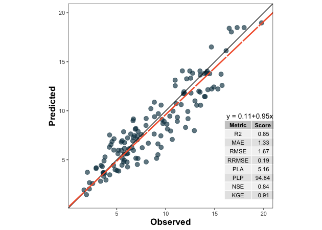
binomial_case <- data.frame(labels = sample(c("Pos","Neg"), 100, replace = TRUE),
                            predictions = sample(c("Pos","Neg"), 100, replace = TRUE)) %>%
  mutate(predictions = as.factor(predictions), labels = as.factor(labels))

multinomial_case <- data.frame(labels = sample(c("Red","Green", "Blue"), 100, replace = TRUE),
                               predictions = sample(c("Red","Green", "Blue"), 100, replace = TRUE) ) %>%
mutate(predictions = as.factor(predictions), labels = as.factor(labels))# a. Print
binomial_case %>% confusion_matrix(obs = labels, pred = predictions,
plot = FALSE, colors = c(low="#f9dbbd" , high="#735d78"),
unit = "count")
#> OBSERVED
#> PREDICTED Neg Pos
#> Neg 24 24
#> Pos 21 31
# b. Plot
binomial_case %>% confusion_matrix(obs = labels, pred = predictions,
plot = TRUE, colors = c(low="#f9dbbd" , high="#735d78"),
unit = "count", print_metrics = TRUE)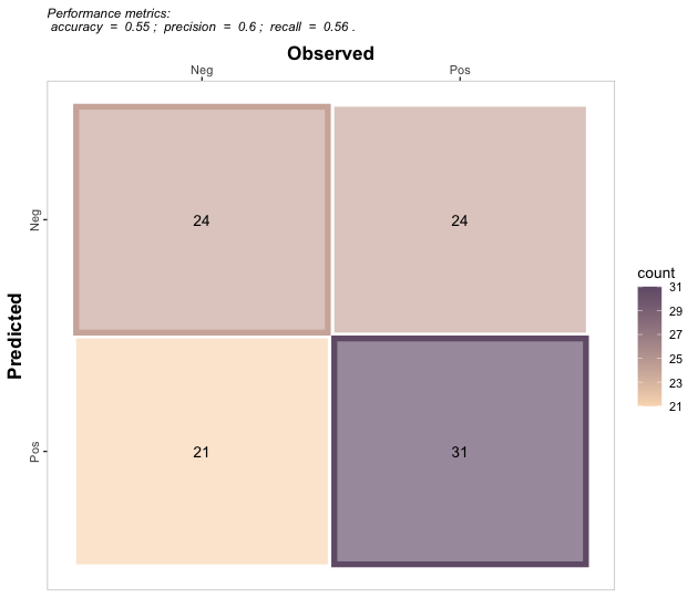
# a. Print
multinomial_case %>% confusion_matrix(obs = labels,
                                      pred = predictions,
                                      plot = FALSE, colors = c(low="#f9dbbd" , high="#735d78"),
                                      unit = "count")
#>          OBSERVED
#> PREDICTED Blue Green Red
#>     Blue     9    11   9
#>     Green   11    12  11
#>     Red     13    13  11

# b. Plot
multinomial_case %>% confusion_matrix(obs = labels,
                                      pred = predictions,
                                      plot = TRUE, colors = c(low="#d3dbbd" , high="#885f78"),
                                      unit = "count", print_metrics = TRUE)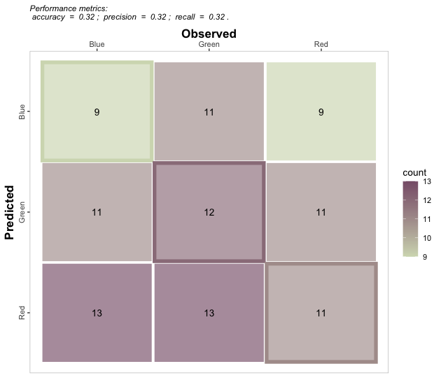
# Get classification metrics one by one
binomial_case %>% accuracy(data = ., obs = labels, pred = predictions, tidy=TRUE)
#>   accuracy
#> 1     0.55
binomial_case %>% error_rate(data = ., obs = labels, pred = predictions, tidy=TRUE)
#>   error_rate
#> 1       0.45
binomial_case %>% precision(data = ., obs = labels, pred = predictions, tidy=TRUE)
#>   precision
#> 1 0.5961538
binomial_case %>% recall(data = ., obs = labels, pred = predictions, atom = F, tidy=TRUE)
#>      recall
#> 1 0.5636364
binomial_case %>% specificity(data = ., obs = labels, pred = predictions, tidy=TRUE)
#>        spec
#> 1 0.5333333
binomial_case %>% balacc(data = ., obs = labels, pred = predictions, tidy=TRUE)
#>      balacc
#> 1 0.5484848
binomial_case %>% fscore(data = ., obs = labels, pred = predictions, tidy=TRUE)
#>      fscore
#> 1 0.5794393
binomial_case %>% agf(data = ., obs = labels, pred = predictions, tidy=TRUE)
#>         agf
#> 1 0.5462663
binomial_case %>% gmean(data = ., obs = labels, pred = predictions, tidy=TRUE)
#>       gmean
#> 1 0.5482755
binomial_case %>% khat(data = ., obs = labels, pred = predictions, tidy=TRUE)
#>         khat
#> 1 0.09638554
binomial_case %>% mcc(data = ., obs = labels, pred = predictions, tidy=TRUE)
#>          mcc
#> 1 0.09656091
binomial_case %>% fmi(data = ., obs = labels, pred = predictions, tidy=TRUE)
#>         fmi
#> 1 0.5796671
binomial_case %>% posLr(data = ., obs = labels, pred = predictions, tidy=TRUE)
#>      posLr
#> 1 1.207792
binomial_case %>% negLr(data = ., obs = labels, pred = predictions, tidy=TRUE)
#>       negLr
#> 1 0.8181818
binomial_case %>% dor(data = ., obs = labels, pred = predictions, tidy=TRUE)
#>       dor
#> 1 1.47619

# Get all at once with metrics_summary()
binomial_case %>% metrics_summary(data = ., obs = labels, pred = predictions, type = "classification")
#>         Metric      Score
#> 1     accuracy 0.55000000
#> 2   error_rate 0.45000000
#> 3    precision 0.59615385
#> 4       recall 0.56363636
#> 5  specificity 0.53333333
#> 6       balacc 0.54848485
#> 7       fscore 0.57943925
#> 8          agf 0.54626632
#> 9        gmean 0.54827553
#> 10        khat 0.09638554
#> 11         mcc 0.09656091
#> 12         fmi 0.57966713
#> 13         bmi 0.09696970
#> 14         csi 0.40789474
#> 15      deltap 0.09615385
#> 16       posLr 1.20779221
#> 17       negLr 0.81818182
#> 18         dor 1.47619048
#> 19         npv 0.50000000
#> 20         FPR 0.46666667
#> 21         FNR 0.43636364
#> 22         FDR 0.40384615
#> 23         FOR 0.50000000
#> 24      preval 0.55000000
#> 25    preval_t 0.49309260
#> 26     AUC_roc 0.54848485
#> 27          p4 0.54595487

# Multinomial
multinomial_case %>% metrics_summary(data = ., obs = labels, pred = predictions, type = "classification")
#> Warning in metrica::fscore(data = ~., obs = ~labels, pred = ~predictions, : For
#> multiclass cases, the fscore should be estimated at a class level. Please,
#> consider using `atom = TRUE`
#> Warning in metrica::agf(data = ~., obs = ~labels, pred = ~predictions,
#> pos_level = pos_level): For multiclass cases, the agf should be estimated at a
#> class level. Please, consider using `atom = TRUE`
#> Warning in metrica::fmi(data = ~., obs = ~labels, pred = ~predictions,
#> pos_level = pos_level): The Fowlkes-Mallows Index is not available for
#> multiclass cases. The result has been recorded as NaN.
#> Warning in metrica::preval(data = ~., obs = ~labels, pred = ~predictions, : For
#> multiclass cases, prevalence should be estimated at a class level. A NaN has
#> been recorded as the result. Please, use `atom = TRUE`
#> Warning in metrica::preval_t(data = ~., obs = ~labels, pred = ~predictions, : For multiclass cases, prevalence threshold should be estimated at a class level.
#>       A NaN has been recorded as the result. Please, use `atom = TRUE`.
#> Warning in metrica::p4(data = ~., obs = ~labels, pred = ~predictions, pos_level
#> = pos_level): Sorry, the p4 metric has not been generalized for multinomial
#> cases. A NaN has been recorded as the result
#>         Metric       Score
#> 1     accuracy  0.32000000
#> 2   error_rate  0.68000000
#> 3    precision  0.32019443
#> 4       recall  0.32029977
#> 5  specificity  0.66031031
#> 6       balacc  0.49030504
#> 7       fscore  0.32024709
#> 8          agf  0.45982261
#> 9        gmean  0.45988829
#> 10        khat -0.01918465
#> 11         mcc -0.01926552
#> 12         fmi         NaN
#> 13         bmi -0.01938991
#> 14         csi  0.13793860
#> 15      deltap -0.01951385
#> 16       posLr  0.94291874
#> 17       negLr  1.02936485
#> 18         dor  0.91601996
#> 19         npv  0.66029172
#> 20         FPR  0.33968969
#> 21         FNR  0.67970023
#> 22         FDR  0.67980557
#> 23         FOR  0.33970828
#> 24      preval         NaN
#> 25    preval_t         NaN
#> 26     AUC_roc  0.49030504
#> 27          p4         NaN

# Get a selected list at once with metrics_summary()
selected_class_metrics <- c("accuracy", "recall", "fscore")

# Binary
binomial_case %>% metrics_summary(data = ., obs = labels, pred = predictions, type = "classification",
                                  metrics_list = selected_class_metrics)
#>     Metric     Score
#> 1 accuracy 0.5500000
#> 2   recall 0.5636364
#> 3   fscore 0.5794393

# Multiclass
multinomial_case %>% metrics_summary(data = ., obs = labels, pred = predictions, type = "classification",
                                  metrics_list = selected_class_metrics)
#> Warning in metrica::fscore(data = ~., obs = ~labels, pred = ~predictions, : For
#> multiclass cases, the fscore should be estimated at a class level. Please,
#> consider using `atom = TRUE`
#> Warning in metrica::agf(data = ~., obs = ~labels, pred = ~predictions,
#> pos_level = pos_level): For multiclass cases, the agf should be estimated at a
#> class level. Please, consider using `atom = TRUE`
#> Warning in metrica::fmi(data = ~., obs = ~labels, pred = ~predictions,
#> pos_level = pos_level): The Fowlkes-Mallows Index is not available for
#> multiclass cases. The result has been recorded as NaN.
#> Warning in metrica::preval(data = ~., obs = ~labels, pred = ~predictions, : For
#> multiclass cases, prevalence should be estimated at a class level. A NaN has
#> been recorded as the result. Please, use `atom = TRUE`
#> Warning in metrica::preval_t(data = ~., obs = ~labels, pred = ~predictions, : For multiclass cases, prevalence threshold should be estimated at a class level.
#>       A NaN has been recorded as the result. Please, use `atom = TRUE`.
#> Warning in metrica::p4(data = ~., obs = ~labels, pred = ~predictions, pos_level
#> = pos_level): Sorry, the p4 metric has not been generalized for multinomial
#> cases. A NaN has been recorded as the result
#>     Metric     Score
#> 1 accuracy 0.3200000
#> 2   recall 0.3202998
#> 3   fscore 0.3202471
multinomial_case %>% accuracy(data = ., obs = labels, pred = predictions, tidy=TRUE)
#>   accuracy
#> 1     0.32
multinomial_case %>% error_rate(data = ., obs = labels, pred = predictions, tidy=TRUE)
#>   error_rate
#> 1       0.68
multinomial_case %>% precision(data = ., obs = labels, pred = predictions, tidy=TRUE)
#>   precision
#> 1 0.3201944
multinomial_case %>% recall(data = ., obs = labels, pred = predictions, atom = F, tidy=TRUE)
#>      recall
#> 1 0.3202998
multinomial_case %>% specificity(data = ., obs = labels, pred = predictions, tidy=TRUE)
#>        spec
#> 1 0.6603103
multinomial_case %>% balacc(data = ., obs = labels, pred = predictions, tidy=TRUE)
#>     balacc
#> 1 0.490305
multinomial_case %>% fscore(data = ., obs = labels, pred = predictions, tidy=TRUE)
#> Warning in fscore(data = ., obs = labels, pred = predictions, tidy = TRUE): For
#> multiclass cases, the fscore should be estimated at a class level. Please,
#> consider using `atom = TRUE`
#>      fscore
#> 1 0.3202471
multinomial_case %>% agf(data = ., obs = labels, pred = predictions, tidy=TRUE)
#> Warning in agf(data = ., obs = labels, pred = predictions, tidy = TRUE): For
#> multiclass cases, the agf should be estimated at a class level. Please,
#> consider using `atom = TRUE`
#>         agf
#> 1 0.4598226
multinomial_case %>% gmean(data = ., obs = labels, pred = predictions, tidy=TRUE)
#>       gmean
#> 1 0.4598883
multinomial_case %>% khat(data = ., obs = labels, pred = predictions, tidy=TRUE)
#>          khat
#> 1 -0.01918465
multinomial_case %>% mcc(data = ., obs = labels, pred = predictions, tidy=TRUE)
#>           mcc
#> 1 -0.01926552
multinomial_case %>% fmi(data = ., obs = labels, pred = predictions, tidy=TRUE)
#> Warning in fmi(data = ., obs = labels, pred = predictions, tidy = TRUE): The
#> Fowlkes-Mallows Index is not available for multiclass cases. The result has
#> been recorded as NaN.
#>   fmi
#> 1 NaN
multinomial_case %>% posLr(data = ., obs = labels, pred = predictions, tidy=TRUE)
#>       posLr
#> 1 0.9429187
multinomial_case %>% negLr(data = ., obs = labels, pred = predictions, tidy=TRUE)
#>      negLr
#> 1 1.029365
multinomial_case %>% dor(data = ., obs = labels, pred = predictions, tidy=TRUE)
#>       dor
#> 1 0.91602
multinomial_case %>% deltap(data = ., obs = labels, pred = predictions, tidy=TRUE)
#>        deltap
#> 1 -0.01951385
multinomial_case %>% csi(data = ., obs = labels, pred = predictions, tidy=TRUE)
#>         csi
#> 1 0.1379386
multinomial_case %>% FPR(data = ., obs = labels, pred = predictions, tidy=TRUE)
#>         FPR
#> 1 0.3396897
multinomial_case %>% FNR(data = ., obs = labels, pred = predictions, tidy=TRUE)
#>         FNR
#> 1 0.6797002
multinomial_case %>% FDR(data = ., obs = labels, pred = predictions, tidy=TRUE)
#>         FDR
#> 1 0.6798056
multinomial_case %>% FOR(data = ., obs = labels, pred = predictions, tidy=TRUE)
#>         FOR
#> 1 0.3397083
multinomial_case %>% preval(data = ., obs = labels, pred = predictions, tidy=TRUE)
#> Warning in preval(data = ., obs = labels, pred = predictions, tidy = TRUE): For
#> multiclass cases, prevalence should be estimated at a class level. A NaN has
#> been recorded as the result. Please, use `atom = TRUE`
#>   prev
#> 1  NaN
multinomial_case %>% preval_t(data = ., obs = labels, pred = predictions, tidy=TRUE)
#> Warning in preval_t(data = ., obs = labels, pred = predictions, tidy = TRUE): For multiclass cases, prevalence threshold should be estimated at a class level.
#>       A NaN has been recorded as the result. Please, use `atom = TRUE`.
#>   preval_t
#> 1      NaN
multinomial_case %>% AUC_roc(data = ., obs = labels, pred = predictions, tidy=TRUE)
#>    AUC_roc
#> 1 0.490305Please, visit the vignette
Thank you for considering contributing to our open-source project.
Although we are not directly funded to maintain metrica, we
care about reproducible science, like you. Thus, all contributions are
more than welcome!
There are multiple ways you can contribute to metrica
such as asking questions, propose ideas, report bugs, improve the
vignettes & documentation of functions, as well as contributing with
code, of course.
For comments, suggestions, and bug reports, we highly encourage to use our GitHub issues section.
To improve the documentation and contribute with code, we encourage to fork the repo and use pull requests to contribute code.
Please note that the metrica project is released with a Contributor Code of Conduct. By contributing to this project, you agree to abide by its terms.