![]()
![]()
netplot is a graph visualization engine for R that
emphasizes aesthetics. Its defaults are chosen so that a single
call to nplot() produces a publication-quality figure out
of the box, while still giving you fine-grained control when you need
it. It works directly with igraph, network,
and adjacency-matrix objects.
Compared with the base plot() methods in
igraph and sna/network, netplot
aims to make the common case beautiful and the hard case
possible:
nplot(g, vertex.color = ~ group, vertex.nsides = ~ group, vertex.size = ~ degree).
Categorical, numeric, and logical attributes are each handled sensibly,
and a legend is added automatically. See
vignette("formulas").grid. Because netplot draws
with the grid system (the same engine as
ggplot2), plots are first-class grid objects: you can
post-edit them with set_vertex_gpar() /
set_edge_gpar(), arrange several with
gridExtra::grid.arrange(), add gradients, and export
cleanly.A quick feature checklist:
The package uses the grid plotting system (just like
ggplot2).
You can install the released version of netplot from CRAN with:
install.packages("netplot")And the development version from GitHub with:
# install.packages("devtools")
devtools::install_github("USCCANA/netplot")This is a basic example which shows you how to solve a common problem:
library(igraph)
#>
#> Attaching package: 'igraph'
#> The following objects are masked from 'package:stats':
#>
#>     decompose, spectrum
#> The following object is masked from 'package:base':
#>
#>     union
library(netplot)
#> Loading required package: grid
#>
#> Attaching package: 'netplot'
#> The following object is masked from 'package:igraph':
#>
#>     ego
set.seed(1)
data("UKfaculty", package = "igraphdata")
l <- layout_with_fr(UKfaculty)
#> This graph was created by an old(er) igraph version.
#> ℹ Call `igraph::upgrade_graph()` on it to use with the current igraph version.
#> For now we convert it on the fly...

plot(UKfaculty, layout = l) # ala igraph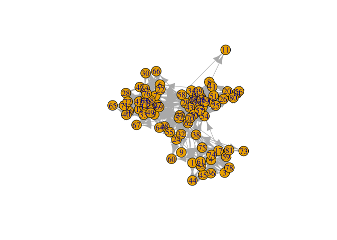
V(UKfaculty)$ss <- runif(vcount(UKfaculty))
nplot(UKfaculty, layout = l) # ala netplot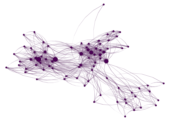
sna::gplot(intergraph::asNetwork(UKfaculty), coord=l)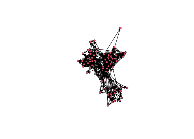
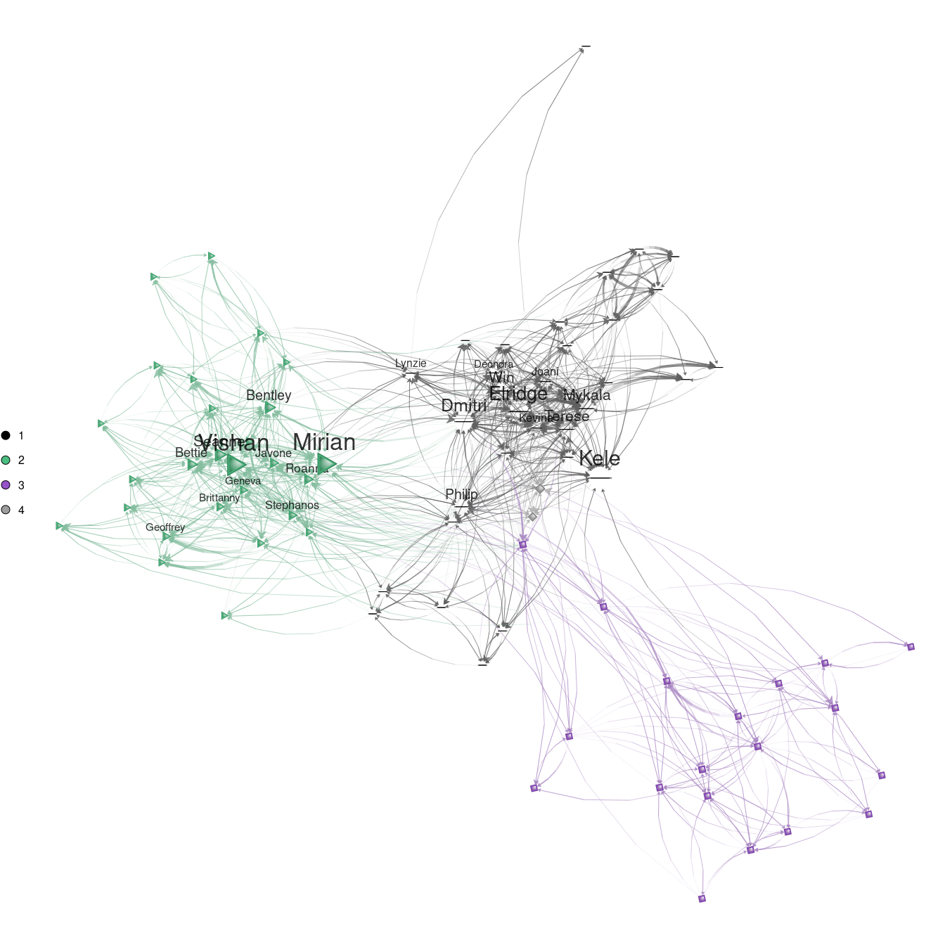
# Random names
set.seed(1)
nam <- sample(babynames::babynames$name, vcount(UKfaculty))

ans <- nplot(
  UKfaculty,
  layout                = l,
  vertex.color          = ~ Group,
  vertex.nsides         = ~ Group,
  vertex.label          = nam,
  vertex.size.range     = c(.01, .03, 4),
  bg.col                = "transparent",
  vertex.label.show     = .25,
  vertex.label.range    = c(10, 25),
  edge.width.range      = c(1, 4, 5),
  vertex.label.fontfamily = "sans"
  )

# Plot it!
ans
Starting version 0.2-0, we can use gradients!
ans |>
  set_vertex_gpar(
    element = "core",
    fill = lapply(get_vertex_gpar(ans, "frame", "col")$col, \(i) {
      radialGradient(c("white", i), cx1=.8, cy1=.8, r1=0)
      }))
# Loading the data
data(USairports, package="igraphdata")
# Generating a layout naively
layout <- V(USairports)$Position
#> This graph was created by an old(er) igraph version.
#> ℹ Call `igraph::upgrade_graph()` on it to use with the current igraph version.
#> For now we convert it on the fly...
layout <- do.call(rbind, lapply(layout, function(x) strsplit(x, " ")[[1]]))
layout[] <- stringr::str_remove(layout, "^[a-zA-Z]+")
layout <- matrix(as.numeric(layout[]), ncol=2)
# Some missingness
layout[which(!complete.cases(layout)), ] <- apply(layout, 2, mean, na.rm=TRUE)
# Have to rotate it (it doesn't matter the origin)
layout <- netplot:::rotate(layout, c(0,0), pi/2)
# Simplifying the network
net <- simplify(USairports, edge.attr.comb = list(
weight = "sum",
name = "concat",
Passengers = "sum",
"ignore"
))
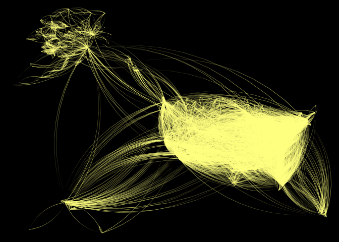
# Pretty graph
nplot(
net,
layout = layout,
edge.width = ~ Passengers,
edge.color = ~
ego(col = "white", alpha = 0) +
alter(col = "yellow", alpha = .75),
skip.vertex = TRUE,
skip.arrows = TRUE,
edge.width.range = c(.75, 4, 4),
bg.col = "black",
edge.line.breaks = 10
)