![]()
![]()
![]()
The goal of protti is to provide flexible functions and workflows for proteomics quality control and data analysis, within a single, user-friendly package. It can be used for label-free DDA, DIA and SRM data generated with search tools and software such as Spectronaut, MaxQuant, Proteome Discoverer and Skyline. Both limited proteolysis mass spectrometry (LiP-MS) and regular bottom-up proteomics experiments can be analysed.
protti is developed and maintained by former members of the lab of Paola Picotti at ETH Zurich. The Picotti lab studies protein structural changes that occur in response to perturbations such as metabolite, drug and protein binding-events, as well as protein aggregation and enzyme activation (Piazza 2018, Piazza 2020, Cappelletti, Hauser & Piazza 2021). We have devoloped mass spectrometry-based structural and chemical proteomic methods aimed at monitoring protein conformational changes in the complex cellular milieu (Feng 2014).
There is a wide range of functions protti provides to the user. The main areas of application are:
The protti package has been peer-reviewed and was published in Bioinformatics Advances:
Jan-Philipp Quast, Dina Schuster, Paola Picotti. protti: an R package for comprehensive data analysis of peptide- and protein-centric bottom-up proteomics data. Bioinformatics Advances, Volume 2, Issue 1, 2022, vbab041, https://doi.org/10.1093/bioadv/vbab041
Please make sure to cite this publication if you used protti for your data analysis.
protti is implemented as an R package.
You can install the release version from CRAN using the
install.packages() function.
install.packages("protti", dependencies = TRUE)You can install the development version from GitHub using the devtools
package by copying the following commands into R:
Note: If you do not have devtools installed make sure to
do so by removing the comment sign (#).
# install.packages("devtools")
devtools::install_github("jpquast/protti", dependencies = TRUE)
The dependencies = TRUE argument in both
install.packages() and
devtools::install_github() also installs suggested packages
that are required for some functions to work. If this argument is not
included functions that use a package that is not installed by default
will throw an error and prompt the user to install the missing package.
If you happen to run into problems during the installation of
protti we recommend removing this argument and
installing packages manually if they are needed for a certain
function.
Since protti is designed to be a flexible tool for the analysis of your data, there are many ways in which it can be used. In this section we will give a general overview for a very simple pipeline that takes a result from the search tool of your choice and in a few steps returns a list of significantly changing proteins or peptides. To ensure that you have your data in the right format please check out the input preparation vignette.
A complete list of functions and their documentation is available here. Within R
you can access the same documentation by calling ? followed
by the function name without parenthesis.
In general functions with the prefix qc_* are used for
quality control of your data. Functions starting with
fetch_* allow you to retrieve data from a database directly
into your R session. When a function starts with filter_*
it is meant to be used to filter your data prior to analysis.
For more in detail workflow suggestions and demonstrations of various functions, you can have a look at the package vignettes. These include:
In this example we are going to analyse synthetic data of which we
know the ground truth. The same principles would apply to any real data.
Before you start analysing your data you should load all required
packages. protti is designed to work well with the tidyverse package family
and we will use them for this example. Therefore, you should also load
them before you get started. Note: If you do not have the
tidyverse installed you can do so by removing the comment
sign (#) in front of the install.packages() function. This
will install them directly from CRAN.
# Load protti
library(protti)

# Install the tidyverse if necessary
# install.packages("tidyverse")

# Load tidyverse packages. Can also be done by calling library(tidyverse)
library(dplyr)
library(magrittr)Usually the search tool of your choice generates a report for you
that has either a .txt or .csv format. You can
easily load reports into R by using the read_protti()
function. This function is a wrapper around the fast
fread() function from the data.table package
and the clean_names() function from the
janitor package. This will allow you to not only load your
data into R very fast, but also to clean up the column names into lower
snake case. This will make it easier to remember them and to use them in
your data analysis.
# Load data
data <- read_protti("filename.csv")
Since we will use synthetic data for this example we are going to
call the create_synthetic_data() function from
protti. Of course you do not need to do this step in
your analysis pipeline.
The data this function creates is similar to data obtained from a LiP-MS experiment. Please note that any of the steps in this workflow can also be applied to protein abundance data that contains protein IDs and protein intensities.
set.seed(42) # Makes example reproducible

# Create synthetic data
data <- create_synthetic_data(
  n_proteins = 100,
  frac_change = 0.05,
  n_replicates = 4,
  n_conditions = 2,
  method = "effect_random",
  additional_metadata = FALSE
)

# The method "effect_random" as opposed to "dose-response" just randomly samples
# the extend of the change of significantly changing peptides for each condition.
# They do not follow any trend and can go in any direction.Before you start analysing your data it is recommended that you filter out any observations not necessary for your analysis. These include for example:
On your own data you can easily achieve this with
dplyr’s filter() function. Our synthetic data
does not require any filtering at this step.
Due to the fact that variances increase with increasing raw
intensities, statistical tests would have a bias towards lower-intensity
peptides or proteins. Therefore you should log2 transform your data to
correct for this mean-variance relationship. We do not need to do this
for the synthetic data as it is already log2 transformed. For your own
data just use dplyr’s mutate() together with
log2().
In addition to filtering and log2 transformation it is also advised
to normalise your data to equal out small differences in overall sample
intensities that result from unequal sample concentrations.
protti provides the normalise() function
for this purpose. For this example we will use median normalisation
(method = "median"). This function generates an additional
column called normalised_intensity_log2 that contains the
normalised intensities.
Note: If your search tool already normalised your data you should not normalise it another time.
normalised_data <- data %>%
  normalise(
    sample = sample,
    intensity_log2 = peptide_intensity_missing,
    method = "median"
)The next step is to deal with missing data points. You could choose
to impute missing data in a later step, but this is only recommended if
only a small proportion of your data is missing. In order to calculate
statistical significance of differentially abundant peptides or proteins
we would like to have at least a minimum number of observations per
condition. The protti function
assign_missingness() checks for each treatment-to-reference
condition if the defined minimum number of observations is satisfied and
assigns a missingness type to each comparison as follows.
If a certain condition has all replicates while the other one has
less than 20% (adjusted downward) of total possible replicates, the case
is considered to be “missing not at random” (MNAR). In
order to be labeled “missing at random” (MAR) 70% (adjusted
downward) of total replicates need to be present in both conditions. If
you performed an experiment with 4 replicates that means that both
conditions need to contain at least 2 observations. Comparisons that
have too few observations are labeled NA. These will not be
imputed if imputation is performed later on using the
impute() function. You can read the exact details in the
documentation of this function and also adjust the thresholds if you
want to be more or less conservative with how many data points to
retain.
data_missing <- normalised_data %>%
  assign_missingness(
    sample = sample,
    condition = condition,
    grouping = peptide,
    intensity = normalised_intensity_log2,
    ref_condition = "condition_1",
    retain_columns = c(protein, change_peptide)
  )

# Next to the columns it generates, assign_missingness only contains the columns
# you provide as input in its output. If you want to retain additional columns you
# can provide them in the retain_columns argument.
Note: Instead of “peptide” in the grouping argument
you can provide protein IDs in case you are working with protein
abundance data. However, then intensities should be protein intensities
and not peptide intensities.
For the calculation of abundance changes and the associated
significances protti provides the function
calculate_diff_abundance(). You can choose between
different statistical methods. For this example we will chose a
moderated t-test.
The type of missingness assigned to a comparison does not have any
influence on the statistical test. However, by default (can be changed)
comparisons with missingness NA are filtered out prior to
p-value adjustment. This means that in addition to imputation, the user
can use missingness cutoffs also in order to define which comparisons
are too incomplete to be trustworthy even if significant.
result <- data_missing %>%
calculate_diff_abundance(
sample = sample,
condition = condition,
grouping = peptide,
intensity_log2 = normalised_intensity_log2,
missingness = missingness,
comparison = comparison,
filter_NA_missingness = TRUE,
method = "moderated_t-test",
retain_columns = c(protein, change_peptide)
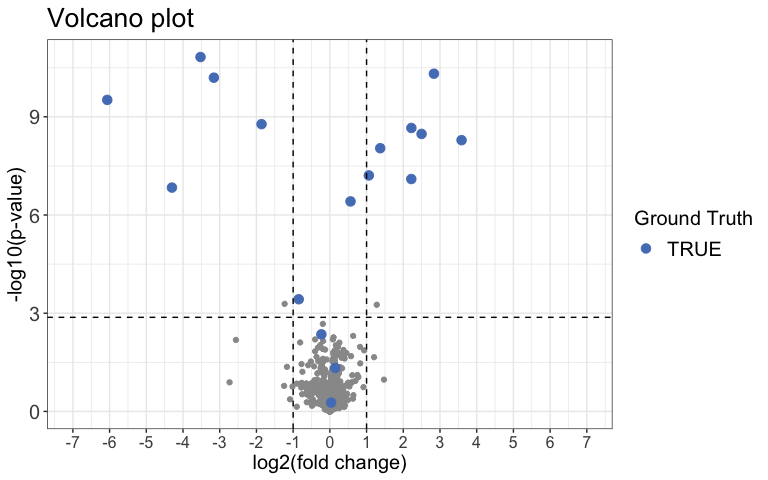
)Next we can use a Volcano plot to visualize significantly changing
peptides with the function volcano_plot(). You can choose
to create an interactive plot with the interactive
argument. Please note that this is not recommended for large
datasets.
result %>%
  volcano_plot(
    grouping = peptide,
    log2FC = diff,
    significance = pval,
    method = "target",
    target_column = change_peptide,
    target = TRUE,
    legend_label = "Ground Truth",
    significance_cutoff = c(0.05, "adj_pval")
  )