


![]()
![]()
qtl2pleio is a software package for use with the R statistical computing
environment. qtl2pleio is freely available for download
and use. I share it under the MIT license.
The user will also want to download and install the qtl2 R package.
We eagerly welcome contributions to qtl2pleio. All pull
requests will be considered. Features requests and bug reports may be
filed as Github issues. All contributors must abide by the code
of conduct.
For technical support, please open a Github issue. If you’re just
getting started with qtl2pleio, please examine the
vignettes. You can also email
frederick.boehm@sdstate.edu
for assistance.
The goal of qtl2pleio is, for a pair of traits that show
evidence for a QTL in a common region, to distinguish between pleiotropy
(the null hypothesis, that they are affected by a common QTL) and the
alternative that they are affected by separate QTL. It extends the
likelihood ratio test of Jiang and Zeng
(1995) for multiparental populations, such as Diversity Outbred
mice, including the use of multivariate polygenic random effects to
account for population structure. qtl2pleio data structures
are those used in the rqtl/qtl2 package.
To install qtl2pleio, use install_github() from the devtools package.
install.packages("qtl2pleio")You may also wish to install the R/qtl2. We will use it below.
install.packages("qtl2")Below, we walk through an example analysis with Diversity Outbred
mouse data. We need a number of preliminary steps before we can perform
our test of pleiotropy vs. separate QTL. Many procedures rely on the R
package qtl2. We first load the qtl2 and
qtl2pleio packages.
library(qtl2)
library(qtl2pleio)
library(ggplot2)qtl2data repository on githubWe’ll consider the DOex
data in the qtl2data
repository. We’ll download the DOex.zip file before calculating founder
allele dosages.
file <- paste0("https://raw.githubusercontent.com/rqtl/",
               "qtl2data/master/DOex/DOex.zip")
DOex <- read_cross2(file)
probs <- calc_genoprob(DOex)Let’s calculate the founder allele dosages from the 36-state genotype probabilities.
pr <- genoprob_to_alleleprob(probs)We now have an allele probabilities object stored in
pr.
names(pr)
#> [1] "2" "3" "X"
dim(pr$`2`)
#> [1] 261   8 127
We see that pr is a list of 3 three-dimensional arrays -
one array for each of 3 chromosomes.
For our statistical model, we need a kinship matrix. We get one with
the calc_kinship function in the rqtl/qtl2
package.
kinship <- calc_kinship(probs = pr, type = "loco")We use the multivariate linear mixed effects model:
\[ \text{vec}(Y) = X \text{vec}(B) + \text{vec}(G) + \text{vec}(E) \]
where \(Y\) contains phenotypes, X contains founder allele probabilities and covariates, and B contains founder allele effects. G is the polygenic random effects, while E is the random errors. We provide more details in the vignette.
qtl2pleio::sim1The function to simulate phenotypes in qtl2pleio is
sim1.
# set up the design matrix, X
pp <- pr[[2]] #we'll work with Chr 3's genotype data
#Next, we prepare a design matrix X
X <- gemma2::stagger_mats(pp[ , , 50], pp[ , , 50])# assemble B matrix of allele effects
B <- matrix(data = c(-1, -1, -1, -1, 1, 1, 1, 1, -1, -1, -1, -1, 1, 1, 1, 1), nrow = 8, ncol = 2, byrow = FALSE)
# set.seed to ensure reproducibility
set.seed(2018-01-30)
Sig <- calc_Sigma(Vg = diag(2), Ve = diag(2), kinship = kinship[[2]])
# call to sim1
Ypre <- sim1(X = X, B = B, Sigma = Sig)
Y <- matrix(Ypre, nrow = 261, ncol = 2, byrow = FALSE)
rownames(Y) <- rownames(pp)
colnames(Y) <- c("tr1", "tr2")Let’s perform univariate QTL mapping for each of the two traits in the Y matrix.
s1 <- scan1(genoprobs = pr, pheno = Y, kinship = kinship)Here is a plot of the results.
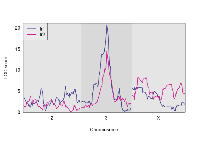
And here are the observed QTL peaks with LOD > 8.
find_peaks(s1, map = DOex$pmap, threshold=8)
#>   lodindex lodcolumn chr       pos       lod
#> 1        1       tr1   3  82.77806 16.287629
#> 2        2       tr2   3  82.77806 15.035673
#> 3 2 tr2 X 128.06510 9.007418We now have the inputs that we need to do a pleiotropy vs. separate
QTL test. We have the founder allele dosages for one chromosome,
i.e., Chr 3, in the R object pp, the matrix of two
trait measurements in Y, and a LOCO-derived kinship matrix,
kinship[[2]].
out <- suppressMessages(scan_pvl(probs = pp,
                pheno = Y,
                kinship = kinship[[2]], # 2nd entry in kinship list is Chr 3
                start_snp = 38,
                n_snp = 25
))To visualize results from our two-dimensional scan, we calculate
profile LOD for each trait. The code below makes use of the R package
ggplot2 to plot profile LODs over the scan region.
library(dplyr)
out %>%
  calc_profile_lods() %>%
  add_pmap(pmap = DOex$pmap$`3`) %>%
  ggplot() + geom_line(aes(x = marker_position, y = profile_lod, colour = trait))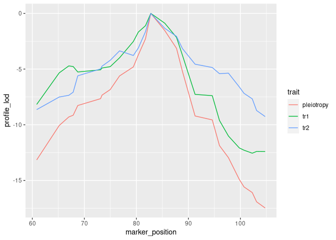
We use the function calc_lrt_tib to calculate the
likelihood ratio test statistic value for the specified traits and
specified genomic region.
(lrt <- calc_lrt_tib(out))
#> [1] 0Before we call boot_pvl, we need to identify the index
(on the chromosome under study) of the marker that maximizes the
likelihood under the pleiotropy constraint. To do this, we use the
qtl2pleio function find_pleio_peak_tib.
(pleio_index <- find_pleio_peak_tib(out, start_snp = 38))
#> log10lik13
#> 50set.seed(2018-11-25) # set for reproducibility purposes.
b_out <- suppressMessages(boot_pvl(probs = pp,
pheno = Y,
pleio_peak_index = pleio_index,
kinship = kinship[[2]], # 2nd element in kinship list is Chr 3
nboot = 10,
start_snp = 38,
n_snp = 25
))(pvalue <- mean(b_out >= lrt))
#> [1] 1citation("qtl2pleio")
#> To cite qtl2pleio in publications use:
#>
#> Boehm FJ, Chesler EJ, Yandell BS, Broman KW (2019) Testing pleiotropy
#> vs. separate QTL in multiparental populations. G3 9:2317-2324
#> doi:10.1534/g3.119.400098
#>
#> A BibTeX entry for LaTeX users is
#>
#> @Article{Boehm2019testing,
#> title = {Testing pleiotropy vs. separate QTL in multiparental populations},
#> author = {Frederick J. Boehm and Elissa J. Chesler and Brian S. Yandell and Karl W. Broman},
#> journal = {G3},
#> year = {2019},
#> volume = {9},
#> issue = {7},
#> pages = {2317-2324},
#> doi = {10.1093/genetics/140.3.1111},
#> url = {https://doi.org/10.1534/g3.119.400098},
#> eprint = {https://academic.oup.com/g3journal/article-pdf/9/7/2317/40667800/g3journal2317.pdf},
#> }