![]()
The R package ‘quantdr’ performs dimension reduction techniques for conditional quantiles by estimating the fewest linear combinations of X that contain all the information on that function. For details of the methodology, see Christou, E. (2020) Central quantile subspace. Statistics and Computing, 30, 677–695.
The main function of the package is cqs, which estimates
the directions of the central quantile subspace. Once the directions are
determined, one can form the new sufficient predictors and estimate the
conditional quantile function using llqr.
dr PackageThe quantdr package includes internal code adapted from
the dr package by Cook,
R. D., & Ni, L. (2005) Sufficient Dimension Reduction via Inverse
Regression: A Minimum Discrepancy Approach. Journal of the American
Statistical Association, 100(470), 410–428, which is no longer
maintained on CRAN.
The original dr package implemented sufficient dimension
reduction methods. We have included any set of essential functions to
support the core functionality of quantdr.
All vendored code has been updated and integrated under the internal
namespace of quantdr.
You can install the released version of quantdr from CRAN with:
install.packages("quantdr") and the development version from GitHub with:
# install.packages("devtools")
devtools::install_github("elianachristou/quantdr")This is a basic example which shows you how to solve the problem.
library(quantdr)

## basic example code - a homoscedastic single-index model

# Setting
set.seed(1234)
n <- 100
p <- 10
taus <- c(0.1, 0.25, 0.5, 0.75, 0.9)
x <- matrix(rnorm(n * p), n, p)
error <- rnorm(n)
y <- 3 * x[, 1] + x[, 2] + error

# true direction that spans each central quantile subspace
beta_true <- c(3, 1, rep(0, p - 2))
beta_true / sqrt(sum(beta_true^2))
#>  [1] 0.9486833 0.3162278 0.0000000 0.0000000 0.0000000 0.0000000 0.0000000
#>  [8] 0.0000000 0.0000000 0.0000000

# sufficient direction
dir1 <- x %*% beta_true

# Estimate the directions of each central quantile subspace
# Since dtau is known to be one, the algorithm will produce only one vector
out <- matrix(0, p, length(taus))
for (i in 1:length(taus)) {
  out[, i] <- cqs(x, y, tau = taus[i], dtau = 1)$qvectors
}
out
#>               [,1]         [,2]         [,3]        [,4]         [,5]
#>  [1,]  0.955128387  0.953563098  0.952948139  0.95432205  0.957157424
#>  [2,]  0.282221145  0.286814969  0.287974471  0.28469153  0.275583662
#>  [3,]  0.040025231  0.040124118  0.042667367  0.04252055  0.039230711
#>  [4,]  0.037794516  0.037393312  0.038590479  0.03742298  0.037849461
#>  [5,] -0.002145479 -0.002710592 -0.003885815 -0.00284509  0.002339282
#>  [6,] -0.049903668 -0.047392988 -0.042769158 -0.05199378 -0.053432303
#>  [7,]  0.029549555  0.029730897  0.028417264  0.02857128  0.032300729
#>  [8,]  0.016985520  0.017341603  0.018789922  0.01678999  0.017397007
#>  [9,]  0.015690746  0.019725351  0.023914784  0.01175831  0.009852825
#> [10,]  0.033877447  0.040239263  0.045541197  0.03261534  0.025062461

# compare each estimated direction with the true one using the angle between the two subspaces
library(pracma)
for (i in 1:length(taus)) {
print(subspace(out[, i], beta_true) / (pi / 2)) # the angle is measured in radians, so divide by pi/2
  }
#> [1] 0.0613477
#> [1] 0.06156084
#> [1] 0.06297377
#> [1] 0.06124013
#> [1] 0.06248869

# Estimate and plot the conditional quantile function using the new sufficient predictors
library(ggplot2)
newx <- x %*% out
qhat <- as.null()
for (i in 1:length(taus)) {
  qhat <- c(qhat, llqr(newx[, i], y, tau = taus[i])$ll_est)
}

data1 <- data.frame(rep(dir1, n), rep(y, n), c(newx), rep(taus, each = n), qhat)
names(data1) <- c("dir1", "y", "newx", "quantiles", 'qhat')
ggplot(data1, aes(x = dir1, y = y)) + geom_point(size = 1) +
  geom_point(aes(x = dir1, qhat), colour = 'red', size = 1) +
  facet_wrap(~quantiles, ncol = 3) + xlab('sufficient direction')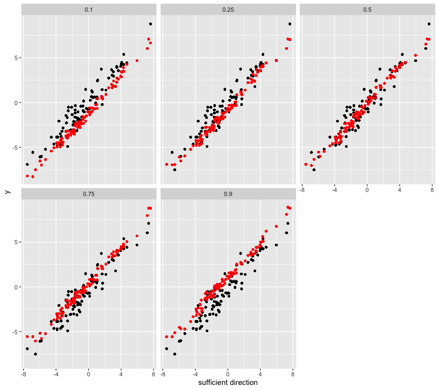
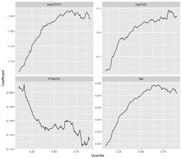
Another example using the Boston housing data from the
MASS library in R.
library(MASS)
attach(Boston)
# read the data
y <- medv
x <- cbind(rm, log(tax), ptratio, log(lstat))
n <- length(y)
p <- dim(x)[2]

# plot the estimated coefficient of each predictor variable for multiple quantiles
tau <- seq(0.1, 0.9, by = 0.005)
beta_hat <- matrix(0, p, length(tau))

for (k in 1:length(tau)) {
  out <- cqs(x, y, tau = tau[k])
  beta_hat[, k] <- out$qvectors[, 1:out$dtau] # the suggested dimension of the central quantile subspace is 1
}

data2 <- data.frame(c(t(beta_hat)), rep(tau, p), rep(c('RM', 'log(TAX)', 'PTRATIO', 'log(LSTAT)'), each = length(tau)))
names(data2) <- c('beta_hat', 'tau', 'coefficient')
ggplot(data2, aes(x = tau, y = beta_hat)) + geom_line() +
  facet_wrap(~coefficient, ncol = 2, scales = "free_y") +
  ylab('Coefficient') + xlab('Quantile')