An R package for estimating risk differences and relative risk measures.
The riskCommunicator package facilitates the estimation
of common epidemiological effect measures that are relevant to public
health, but that are often not trivial to obtain from common regression
models, like logistic regression. In particular,
riskCommunicator estimates risk and rate differences, in
addition to risk and rate ratios. The package estimates these effects
using g-computation with the appropriate parametric model depending on
the outcome (logistic regression for binary outcomes, Poisson regression
for rate or count outcomes, negative binomial regression for
overdispersed rate or count outcomes, and linear regression for
continuous outcomes). Therefore, the package can handle binary, rate,
count, and continuous outcomes and allows for dichotomous, categorical
(>2 categories), or continuous exposure variables. Additional
features include estimation of effects stratified by subgroup and
adjustment of standard errors for clustering. Confidence intervals are
constructed by bootstrap at the individual or cluster level, as
appropriate.
This package operationalizes g-computation, which has not been widely
adopted due to computational complexity, in an easy-to-use
implementation tool to increase the reporting of more interpretable
epidemiological results. To make the package accessible to a broad range
of health researchers, our goal was to design a function that was as
straightforward as the standard logistic regression functions in R
(e.g. glm) and that would require little to no expertise in
causal inference methods or advanced coding.
You can install the released version of riskCommunicator
from CRAN with:
install.packages("riskCommunicator")The development version is available as a source package through GitHub. Installation requires the ability to compile R packages. This means that R and the R tool-chain must be installed, which requires the Xcode command-line tools on Mac and Rtools on Windows.
The easiest source installation method uses the devtools package:
# install.packages("devtools")
devtools::install_github("jgrembi/riskCommunicator")Bugs and difficulties in using riskCommunicator are
welcome on the issue tracker.
Planned feature improvements are also publicly catalogued on the
“Issues” page for riskCommunicator: https://github.com/jgrembi/riskCommunicator/issues
This is a basic example which shows you how to answer the following question: What is the effect of obesity on the 24-year risk of cardiovascular disease or death due to any cause?
In this example, we specify obesity as a categorical variable
(bmicat coding: 0 = normal weight; 1=underweight;
2=overweight; 3=obese)
library(riskCommunicator)
library(ggplot2)
library(tidyverse)
#> ── Attaching packages ─────────────────────────────────────── tidyverse 1.3.1 ──
#> ✔ tibble  3.1.7     ✔ dplyr   1.0.9
#> ✔ tidyr   1.2.0     ✔ stringr 1.4.0
#> ✔ readr   2.1.2     ✔ forcats 0.5.1
#> ✔ purrr   0.3.4
#> ── Conflicts ────────────────────────────────────────── tidyverse_conflicts() ──
#> ✖ dplyr::filter() masks stats::filter()
#> ✖ dplyr::lag()    masks stats::lag()
## basic example code
data(cvdd)
set.seed(345)
bmi.results <- gComp(data = cvdd, Y = "cvd_dth", X = "bmicat", Z = c("AGE", "SEX", "DIABETES", "CURSMOKE", "PREVHYP"), outcome.type = "binary", R = 200)
summary(bmi.results)
#> Formula:
#> cvd_dth ~ bmicat + AGE + SEX + DIABETES + CURSMOKE + PREVHYP
#>
#> Family: binomial
#> Link function: logit
#>
#> Contrast: bmicat1 v. bmicat0 bmicat2 v. bmicat0 bmicat3 v. bmicat0
#>
#> Parameter estimates:
#>                             bmicat1_v._bmicat0 Estimate (95% CI)
#> Risk Difference                            0.042 (-0.082, 0.178)
#> Risk Ratio                                  1.106 (0.792, 1.454)
#> Odds Ratio                                  1.248 (0.631, 2.506)
#> Number needed to treat/harm                               23.846
#>                             bmicat2_v._bmicat0 Estimate (95% CI)
#> Risk Difference                            0.017 (-0.005, 0.049)
#> Risk Ratio                                  1.044 (0.988, 1.126)
#> Odds Ratio                                  1.097 (0.973, 1.297)
#> Number needed to treat/harm                               57.405
#>                             bmicat3_v._bmicat0 Estimate (95% CI)
#> Risk Difference                             0.093 (0.056, 0.136)
#> Risk Ratio                                  1.235 (1.143, 1.354)
#> Odds Ratio                                  1.628 (1.348, 2.037)
#> Number needed to treat/harm                               10.733
#>
#> Underlying glm:
#> Call:  stats::glm(formula = formula, family = family, data = working.df,
#>     na.action = stats::na.omit)
#>
#> Coefficients:
#> (Intercept)      bmicat1      bmicat2      bmicat3          AGE         SEX1
#>    -5.73445      0.22184      0.09288      0.48711      0.10305     -0.80522
#>   DIABETES1    CURSMOKE1     PREVHYP1
#>     1.50504      0.59057      0.76174
#>
#> Degrees of Freedom: 4220 Total (i.e. Null);  4212 Residual
#>   (19 observations deleted due to missingness)
#> Null Deviance:       5735
#> Residual Deviance: 4686  AIC: 4704
The results from the g-computation show the estimated risk difference and ratio, in addition to other information. From these results, we see that obese persons have an 11.6% (95% CI: 7.2, 16.6) increase in 24-year risk of cardiovascular disease or death compared to normal weight persons. Underweight persons also have increased risk, more so than overweight persons. Not surprisingly, the estimate comparing underweight to normal weight persons is imprecise given the few people in the dataset who were underweight.
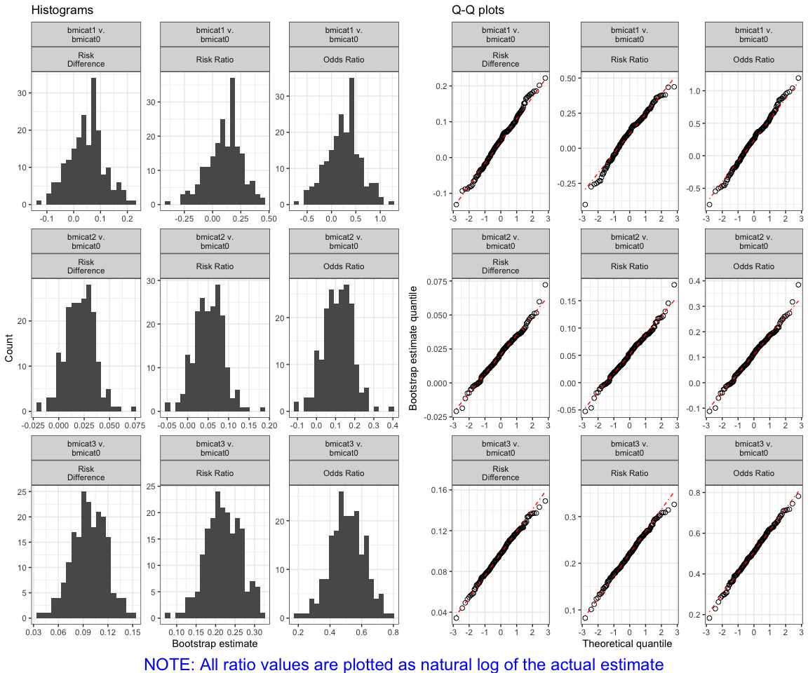
You can verify that the parameter estimates from the bootstraps are normally distributed:
plot(bmi.results)
#> Warning in log(as.numeric(.data$value)): NaNs produced
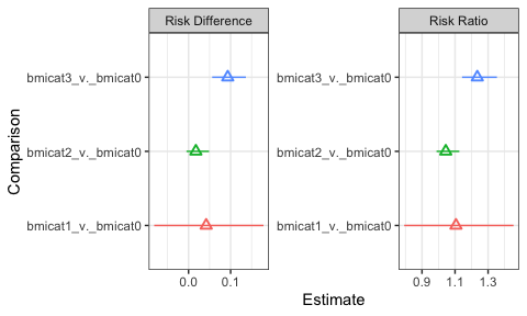
You can also easily plot the outcome estimates:
ggplot(bmi.results$results.df %>%
         filter(Parameter %in% c("Risk Difference", "Risk Ratio"))
) +
  geom_pointrange(aes(x = Comparison,
                      y = Estimate,
                      ymin = `2.5% CL`,
                      ymax = `97.5% CL`,
                      color = Comparison),
                  shape = 2
  ) +
  coord_flip() +
  facet_wrap(~Parameter, scale = "free") +
  theme_bw() +
  theme(legend.position = "none")