
![]()
![]()
rwhatsapp is a small yet robust package that provides
some infrastructure to work with WhatsApp text data in
R.
WhatsApp seems to become increasingly important not just as a
messaging service but also as a social network—thanks to its group chat
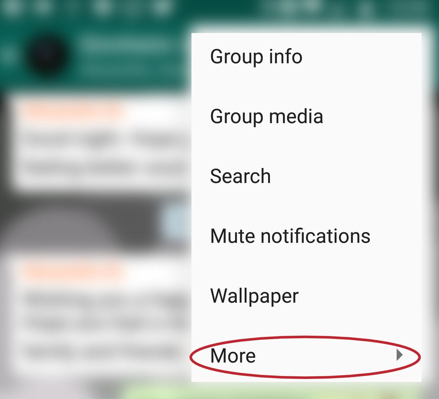
capabilities. Furthermore, retrieving chat logs from the Android or iOS
app is very straightforward: Simply choose More in the menu
of a chat, then Export chat and export the history to a txt
file.


This package is intended to make the first step of analysing WhatsApp
text data as easy as possible: reading your chat history into
R. This should work, no matter which device or locale you
used to retrieve the txt or zip file
containing your conversations.
If you have ideas for what can be useful functions or if you have problems with an existing function, please don’t hesitate to file an issue report.
install.packages("rwhatsapp")Or install the GitHub version:
remotes::install_github("JBGruber/rwhatsapp")The package comes with a small sample that you can use to get going.
history <- system.file("extdata", "sample.txt", package = "rwhatsapp")The main function of the package, rwa_read() can handle
txt (and zip) files directly, which means that
you can simply provide the path to a file to get started:
library("rwhatsapp")
chat <- rwa_read(history)
chat
#> # A tibble: 9 x 6
#> time author text source emoji emoji_name
#> <dttm> <fct> <chr> <chr> <lis> <list>
#> 1 2017-07-12 22:35:56 <NA> "Messages to th… /home/johannes… <NUL… <NULL>
#> 2 2017-07-12 22:35:56 <NA> "You created gr… /home/johannes… <NUL… <NULL>
#> 3 2017-07-12 22:35:56 Johanne… "<Media omitted… /home/johannes… <NUL… <NULL>
#> 4 2017-07-12 22:35:56 Johanne… "Fruit bread wi… /home/johannes… <chr… <chr [2]>
#> 5 2017-07-13 09:12:56 Test "It's fun doing… /home/johannes… <NUL… <NULL>
#> 6 2017-07-13 09:16:56 Johanne… "Haha it sure i… /home/johannes… <chr… <chr [1]>
#> 7 2018-09-28 13:27:56 Johanne… "Did you know t… /home/johannes… <NUL… <NULL>
#> 8 2018-09-28 13:28:56 Johanne… "😀😃😄😁😆😅😂🤣☺😊😇🙂🙃😉… /home/johannes… <chr… <chr [242…
#> 9 2018-09-28 13:30:56 Johanne… "🤷♀🤷🏻♂🙎♀🙎♂🙍… /home/johannes… <chr… <chr [87]>Now, this isn’t very interesting so you will probably want to use your own data. For this demonstration, I use one of my own chat logs from a conversation with friends:[1]
library("dplyr")
chat <- rwa_read("/home/johannes/WhatsApp Chat.txt") %>%
  filter(!is.na(author)) # remove messages without author
chat
#> # A tibble: 16,814 x 6
#>    time                author   text                source      emoji emoji_name
#>    <dttm>              <fct>    <chr>               <chr>       <lis> <list>
#>  1 2015-12-10 19:57:56 Artur K… <Media omitted>     /home/joha… <NUL… <NULL>
#>  2 2015-12-10 22:31:56 Erika I… 😂😂😂😂😂😂        /home/joha… <chr… <chr [6]>
#>  3 2015-12-11 02:13:56 Alexand… 🙈                  /home/joha… <chr… <chr [1]>
#>  4 2015-12-11 02:23:56 Johanne… 😂                  /home/joha… <chr… <chr [1]>
#>  5 2015-12-11 02:24:56 Johanne… Die Petitionen Tru… /home/joha… <chr… <chr [1]>
#>  6 2015-12-11 03:51:56 Erika I… Läääuft             /home/joha… <NUL… <NULL>
#>  7 2015-12-12 07:49:56 Johanne… <Media omitted>     /home/joha… <NUL… <NULL>
#>  8 2015-12-12 07:53:56 Erika I… was macht ihr huet… /home/joha… <NUL… <NULL>
#>  9 2015-12-12 07:55:56 Johanne… Alex arbeitet weil… /home/joha… <NUL… <NULL>
#> 10 2015-12-12 07:55:56 Johanne… und ich spiele auf… /home/joha… <NUL… <NULL>
#> # … with 16,804 more rows
You can see from the size of the resulting data.frame
that we write a lot in this group! Let’s see over how much time we
managed to accumulate 16,814 messages. I use a couple of extra packages
for that:
library("ggplot2"); theme_set(theme_minimal())
library("lubridate")
chat %>%
  mutate(day = date(time)) %>%
  count(day) %>%
  ggplot(aes(x = day, y = n)) +
  geom_bar(stat = "identity") +
  ylab("") + xlab("") +
  ggtitle("Messages per day")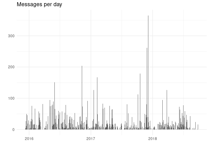
The chat has been going on for a while and on some days there were more than a hundred messages. Who’s responsible for all of this?
chat %>%
  mutate(day = date(time)) %>%
  count(author) %>%
  ggplot(aes(x = reorder(author, n), y = n)) +
  geom_bar(stat = "identity") +
  ylab("") + xlab("") +
  coord_flip() +
  ggtitle("Number of messages")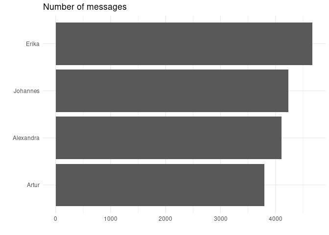
Looks like we contributed more or less the same number of messages, with Erika slightly leading the field.
One thing that is always fun to do is finding out what people’s favourite emojis are:
library("tidyr")
chat %>%
  unnest(emoji) %>%
  count(author, emoji, sort = TRUE) %>%
  group_by(author) %>%
  top_n(n = 6, n) %>%
  ggplot(aes(x = reorder(emoji, n), y = n, fill = author)) +
  geom_col(show.legend = FALSE) +
  ylab("") +
  xlab("") +
  coord_flip() +
  facet_wrap(~author, ncol = 2, scales = "free_y")  +
  ggtitle("Most often used emojis")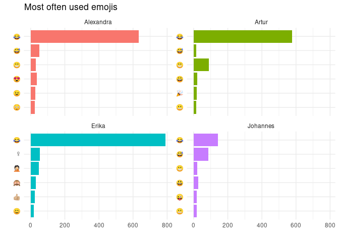
On some operating systems, the default font in ggplot2
does not support emojis. In this case you might want to move the emojis
inside the plot instead. I use emoji images from Twitter as they can be
easily queried:
library("ggimage")
emoji_data <- rwhatsapp::emojis %>% # data built into package
  mutate(hex_runes1 = gsub("\\s.*", "", hex_runes)) %>% # ignore combined emojis
  mutate(emoji_url = paste0("https://abs.twimg.com/emoji/v2/72x72/",
                            tolower(hex_runes1), ".png"))

chat %>%
  unnest(emoji) %>%
  count(author, emoji, sort = TRUE) %>%
  group_by(author) %>%
  top_n(n = 6, n) %>%
  left_join(emoji_data, by = "emoji") %>%
  ggplot(aes(x = reorder(emoji, n), y = n, fill = author)) +
  geom_col(show.legend = FALSE) +
  ylab("") +
  xlab("") +
  coord_flip() +
  geom_image(aes(y = n + 20, image = emoji_url)) +
  facet_wrap(~author, ncol = 2, scales = "free_y") +
  ggtitle("Most often used emojis") +
  theme(axis.text.y = element_blank(),
        axis.ticks.y = element_blank())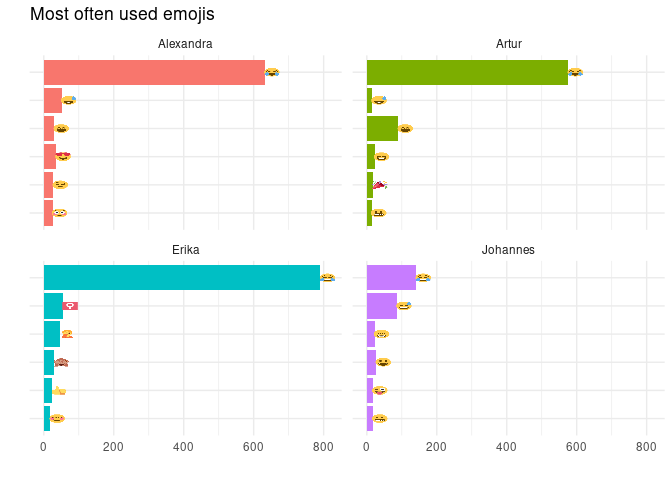
Looks like we have a clear winner: all of us like the :joy: (“face with tears of joy”) most. :sweat_smile: (“grinning face with sweat”) is also very popular, except with Erika who has a few more flamboyant favourites. I apparently tend to use fewer emojis overall while Erika is leading the field (again). (Note that the emojis are not ordered within the facets but by overall number of appearances, see next plot for a solution.)
How does it look if we compare favourite words? I use the excellent
tidytext package to get this task done[2]:
library("tidytext")
chat %>%
  unnest_tokens(input = text,
                output = word) %>%
  count(author, word, sort = TRUE) %>%
  group_by(author) %>%
  top_n(n = 6, n) %>%
  ggplot(aes(x = reorder_within(word, n, author), y = n, fill = author)) +
  geom_col(show.legend = FALSE) +
  ylab("") +
  xlab("") +
  coord_flip() +
  facet_wrap(~author, ncol = 2, scales = "free_y") +
  scale_x_reordered() +
  ggtitle("Most often used words")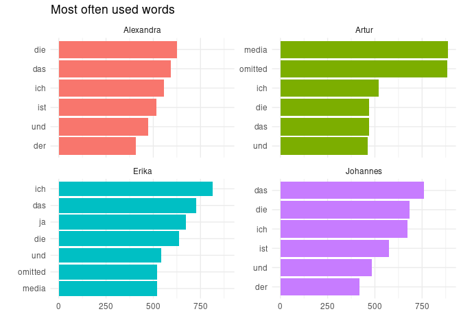
This doesn’t make much sense. First of all, because we write in German which you might not understand :wink:. But it also looks weird that Artur and Erika seem to often use the words “media” and “omitted”. Of course, this is just the placeholder WhatsApp puts into the log file instead of a picture or video. But the other words don’t look particularly useful either. They are what’s commonly called stopwords: words that are used often but don’t carry any substantial meaning. “und” for example is simply “and” in English. “der”, “die” and “das” all mean “the” in English (which makes German pure joy to learn for an English native speaker :sweat_smile:).
To get around this mess, I remove these words before making the plot again:
library("stopwords")
to_remove <- c(stopwords(language = "de"),
               "media",
               "omitted",
               "ref",
               "dass",
               "schon",
               "mal",
               "android.s.wt")

chat %>%
  unnest_tokens(input = text,
                output = word) %>%
  filter(!word %in% to_remove) %>%
  count(author, word, sort = TRUE) %>%
  group_by(author) %>%
  top_n(n = 6, n) %>%
  ggplot(aes(x = reorder_within(word, n, author), y = n, fill = author)) +
  geom_col(show.legend = FALSE) +
  ylab("") +
  xlab("") +
  coord_flip() +
  facet_wrap(~author, ncol = 2, scales = "free_y") +
  scale_x_reordered() +
  ggtitle("Most often used words")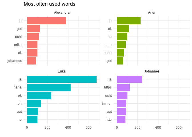
Still not very informative, but hey, this is just a private conversation, what did you expect? It seems though that we agree with each other a lot, as “ja” (yes) and ok are among the top words for all of us. The antonym “ne” (nope) is far less common and only on Artur’s and Erika’s top lists. I seem to send a lot of links as both “https” and “ref” appear on my top list. Alexandra is talking to or about Erika and me pretty often and Artur is the only one who mentions “euro” (as in the currency) pretty often.
Another way to determine favourite words is to calculate the term frequency–inverse document frequency (tf–idf). Basically, what the measure does, in this case, is to find words that are common within the messages of one author but uncommon in the rest of the messages.
chat %>%
  unnest_tokens(input = text,
                output = word) %>%
  select(word, author) %>%
  filter(!word %in% to_remove) %>%
  mutate(word = gsub(".com", "", word)) %>%
  mutate(word = gsub("^gag", "9gag", word)) %>%
  count(author, word, sort = TRUE) %>%
  bind_tf_idf(term = word, document = author, n = n) %>%
  filter(n > 10) %>%
  group_by(author) %>%
  top_n(n = 6, tf_idf) %>%
  ggplot(aes(x = reorder_within(word, n, author), y = n, fill = author)) +
  geom_col(show.legend = FALSE) +
  ylab("") +
  xlab("") +
  coord_flip() +
  facet_wrap(~author, ncol = 2, scales = "free_y") +
  scale_x_reordered() +
  ggtitle("Important words using tf–idf by author")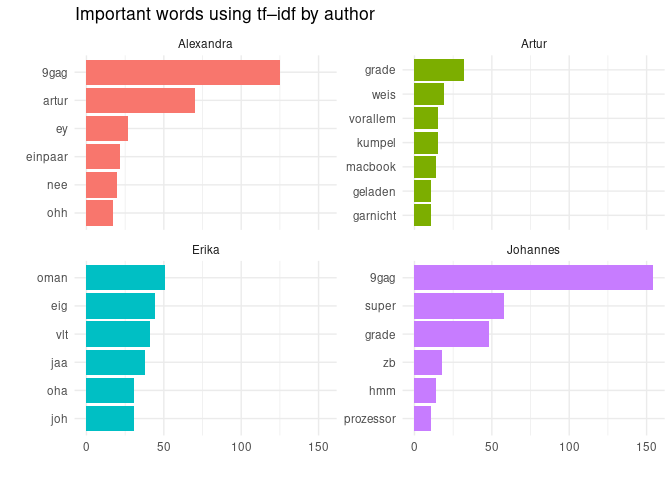
Now the picture changes pretty much entirely. First, the top words of the different authors have very little overlap now compared to before—only exceptions being 9gag (platform to share memes) in Alexandra’s and my messages and “grade” (now) which Artur and I use. This is due to the tf–idf measure which tries to find only words specific to an author.
Now instead of Erika and me, Alexandra talks about Artur, something only she does. Artur is the only one to talk about a Macbook (as he is the only one who owns one). Erika seems to thrive on abbreviations like “oman” (abbreviation for “Oh Mann”/“oh man”, not the country) “eig” (“eigentlich”/actually) “joh” (abbreviation for my name) and curiously “jaa”, which is “ja” (yes) with and unnecessary extra “a”. I show that my favourite adjective is “super” and that I talked about a processor at some point for some reason.
Another common text mining tool is to calculate lexical diversity. Basically, you just check how many unique words are used by an author.
chat %>%
  unnest_tokens(input = text,
                output = word) %>%
  filter(!word %in% to_remove) %>%
  group_by(author) %>%
  summarise(lex_diversity = n_distinct(word)) %>%
  arrange(desc(lex_diversity)) %>%
  ggplot(aes(x = reorder(author, lex_diversity),
                          y = lex_diversity,
                          fill = author)) +
  geom_col(show.legend = FALSE) +
  scale_y_continuous(expand = (mult = c(0, 0, 0, 500))) +
  geom_text(aes(label = scales::comma(lex_diversity)), hjust = -0.1) +
  ylab("unique words") +
  xlab("") +
  ggtitle("Lexical Diversity") +
  coord_flip()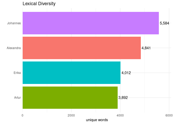
It appears that I use the most unique words, even though Erika wrote more messages overall. Is this because I use some amazing and unique technical terms? Let’s find out:
o_words <- chat %>%
  unnest_tokens(input = text,
                output = word) %>%
  filter(author != "Johannes") %>%
  count(word, sort = TRUE)

chat %>%
  unnest_tokens(input = text,
                output = word) %>%
  filter(author == "Johannes") %>%
  count(word, sort = TRUE) %>%
  filter(!word %in% o_words$word) %>% # only select words nobody else uses
  top_n(n = 6, n) %>%
  ggplot(aes(x = reorder(word, n), y = n)) +
  geom_col(show.legend = FALSE) +
  ylab("") + xlab("") +
  coord_flip() +
  ggtitle("Unique words of Johannes")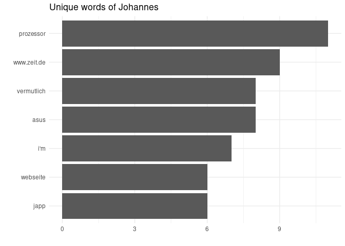
Looking at the top words that are only used by me we see these are words I don’t use very often either. There are two technical terms here: “prozessor” and “webseite” which kind of make sense. I’m also apparently the only one to share links to the German news site zeit.de. The English “i’m” is in there because autocorrect on my phone tends to change the German word “im” (in).
Overall, WhatsApp data is just a fun source to play around with text mining methods. But if you have more serious data, a proper text analysis is also possible, just like with other social media data.
I remove messages with author = NA as these are just
info messages from WhatsApp like “Messages to this group are now
secured with end-to-end encryption. Tap for more info”.
Note that most of the analysis below is taken (or heavily inspired) from the book at tidytextmining.com/ where you can also learn much more about text analysis.