


![]()
The surveyvoi package is a decision support tool for prioritizing sites for ecological surveys based on their potential to improve plans for conserving biodiversity (e.g. plans for establishing protected areas). Given a set of sites that could potentially be acquired for conservation management – wherein some sites have previously been surveyed and other sites have not – this package provides functionality to generate and evaluate plans for additional surveys. Specifically, plans for ecological surveys can be generated using various conventional approaches (e.g. maximizing expected species richness, geographic coverage, diversity of sampled environmental conditions) and by maximizing value of information. After generating plans for surveys, they can also be evaluated using value of information analysis. Please note that several functions depend on the Gurobi optimization software (available from https://www.gurobi.com). Additionally, the JAGS software (available from https://mcmc-jags.sourceforge.io/) is required to fit hierarchical generalized linear models.
The latest official version can be installed from the Comprehensive R Archive Network (CRAN) using the following R code.
install.packages("surveyvoi", repos = "https://cran.rstudio.com/")Alternatively, the latest development version can be installed from GitHub using the following code. Please note that while developmental versions may contain additional features not present in the official version, they may also contain coding errors.
if (!require(remotes)) install.packages("remotes")
remotes::install_github("prioritizr/surveyvoi")The Rtools software needs to be installed to install the surveyvoi R package from source. This software provides system requirements from rwinlib.
The gmp, fftw3, mpfr, and
symphony libraries need to be installed to install the
surveyvoi R package. Although the fftw3 and
symphony libraries are not used directly, they are needed
to successfully install dependencies. For recent versions of Ubuntu
(18.04 and later), these libraries are available through official
repositories. They can be installed using the following system
commands:
apt-get -y update
apt-get install -y libgmp3-dev libfftw3-dev libmpfr-dev coinor-libsymphony-devFor Unix-alikes, gmp (>= 4.2.3), mpfr
(>= 3.0.0), fftw3 (>= 3.3), and symphony
(>= 5.6.16) are required.
The gmp, fftw, mpfr, and
symphony libraries are required. Although the
fftw3 and symphony libraries are not used
directly, they are needed to successfully install dependencies. The
easiest way to install these libraries is using HomeBrew. After installing HomeBrew, these
libraries can be installed using the following commands in the system
terminal:
brew tap coin-or-tools/coinor
brew install symphony
brew install pkg-config
brew install gmp
brew install fftw
brew install mpfrPlease cite the surveyvoi R package when using it in publications. To cite the package, please use:
Hanson, JO, McCune JL, Chadès I, Proctor CA, Hudgins EJ, & Bennett JR (2023) Optimizing ecological surveys for conservation. Journal of Applied Ecology, 60: 41–51. Available at https://doi.org/10.1111/1365-2664.14309.
Here we provide a short example showing how to use the surveyvoi R package to prioritize funds for ecological surveys. In this example, we will generate plans for conducting ecological surveys (termed “survey schemes”) using simulated data for six sites and three conservation features (e.g. bird species). To start off, we will set the seed for the random number generator for reproducibility and load some R packages.
set.seed(502)      # set RNG for reproducibility
library(surveyvoi) # package for value of information analysis
library(dplyr)     # package for preparing data
library(tidyr)     # package for preparing data
library(ggplot2)   # package for plotting data
Now we will load some datasets that are distributed with the package.
First, we will load the sim_sites object. This spatially
explicit dataset (i.e. sf object) contains information on
the sites within our study area. Critically, it contains (i) sites that
have already been surveyed, (ii) candidate sites for additional surveys,
(iii) sites that have already been protected, and (iv) candidate sites
that could be protected in the future. Each row corresponds to a
different site, and each column describes different properties
associated with each site. In this table, the
"management_cost" column indicates the cost of protecting
each site; "survey_cost" column indicates the cost of
conducting an ecological survey within each site; and "e1"
and "e2" columns contain environmental data for each site
(not used in this example). The remaining columns describe the existing
survey data and the spatial distribution of the features across the
sites. The "n1", "n2", and "n3"
columns indicate the number of surveys conducted within each site that
looked for each of the three features (respectively); and
"f1", "f2", and "f3" columns
describe the proportion of surveys within each site that looked for each
feature where the feature was detected (respectively). For example, if
"n1" has a value of 2 and "f1" has a value of
0.5 for a given site, then the feature "f1" was detected in
only one of the two surveys conducted in this site that looked for the
feature. Finally, the "p1", "p2", and
"p3" columns contain modeled probability estimates of each
species being present in each site (see
fit_hglm_occupancy_models() and
fit_xgb_occupancy_models() to generate such estimates for
your own data).
# load data
data(sim_sites)

# print table
print(sim_sites, width = Inf)
## Simple feature collection with 6 features and 13 fields
## Geometry type: POINT
## Dimension: XY
## Bounding box: xmin: 0.02541313 ymin: 0.07851093 xmax: 0.9888107 ymax: 0.717068
## CRS: NA
## # A tibble: 6 × 14
## survey_cost management_cost f1 f2 f3 n1 n2 n3 e1 e2
## <dbl> <dbl> <dbl> <dbl> <dbl> <dbl> <dbl> <dbl> <dbl> <dbl>
## 1 19 99 0 0 0 0 0 0 1.13 0.535
## 2 22 87 0 1 0.25 4 4 4 -1.37 -1.45
## 3 13 94 1 1 0 1 1 1 0.155 -0.867
## 4 19 61 0 0 0 0 0 0 -0.792 1.32
## 5 9 105 0 0 0 0 0 0 -0.194 0.238
## 6 12 136 0 0 0 0 0 0 1.07 0.220
## p1 p2 p3 geometry
## <dbl> <dbl> <dbl> <POINT>
## 1 0.999 0.988 0.21 (0.03529733 0.544939)
## 2 0.001 0.995 0.152 (0.33276 0.3174416)
## 3 0.966 1 0.017 (0.6141922 0.07851093)
## 4 0 0 1 (0.02541313 0.1147132)
## 5 0.11 0.006 0.831 (0.9888107 0.2152785)
## 6 1 1 0.082 (0.9038749 0.717068)# plot cost of protecting each site
ggplot(sim_sites) +
geom_sf(aes(color = management_cost), size = 4) +
ggtitle("management_cost") +
theme(legend.title = element_blank(), text = element_text(size = 16))
# plot cost of conducting an additional survey in each site
# note that these costs are much lower than the protection costs
ggplot(sim_sites) +
geom_sf(aes(color = survey_cost), size = 4) +
ggtitle("survey_cost") +
theme(legend.title = element_blank(), text = element_text(size = 16))
# plot survey data
## n1, n2, n3: number of surveys in each site that looked for each feature
sim_sites %>%
select(n1, n2, n3) %>%
gather(name, value, -geometry) %>%
ggplot() +
geom_sf(aes(color = value), size = 4) +
facet_wrap(~name, nrow = 1) +
theme(text = element_text(size = 16))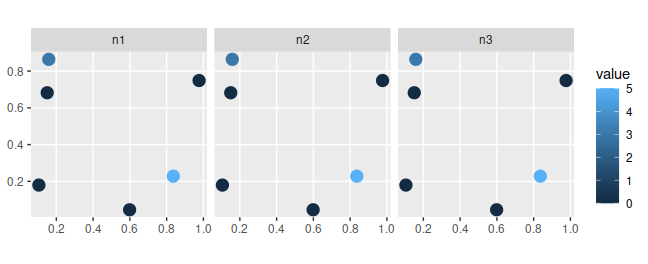
# plot survey results
## f1, f2, f3: proportion of surveys in each site that looked for each feature
##             that detected the feature
sim_sites %>%
select(f1, f2, f3) %>%
gather(name, value, -geometry) %>%
ggplot() +
geom_sf(aes(color = value), size = 4) +
facet_wrap(~name, nrow = 1) +
scale_color_continuous(limits = c(0, 1)) +
theme(text = element_text(size = 16))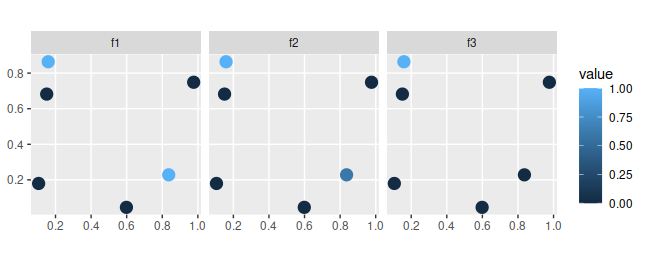
# plot modeled probability of occupancy data
sim_sites %>%
select(p1, p2, p3) %>%
gather(name, value, -geometry) %>%
ggplot() +
geom_sf(aes(color = value), size = 4) +
facet_wrap(~name, nrow = 1) +
scale_color_continuous(limits = c(0, 1)) +
theme(text = element_text(size = 16))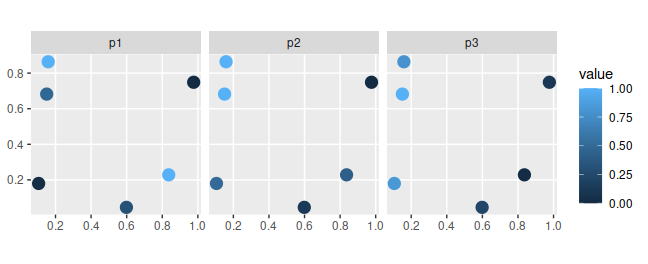
Next, we will load the sim_features object. This table
contains information on the conservation features (e.g. species).
Specifically, each row corresponds to a different feature, and each
column contains information associated with the features. In this table,
the "name" column contains the name of each feature;
"survey" column indicates whether future surveys would look
for this species; "survey_sensitivity" and
"survey_specificity" columns denote the sensitivity (true
positive rate) and specificity (true negative rate) for the survey
methodology for correctly detecting the feature;
"model_sensitivity" and "model_specificity"
columns denote the sensitivity (true positive rate) and specificity
(true negative rate) for the species distribution models fitted for each
feature; and "target" column denotes the required number of
protected sites for each feature (termed “representation target”, each
feature has a target of 2 site).
# load data
data(sim_features)

# print table
print(sim_features, width = Inf)
## # A tibble: 3 × 7
## name survey survey_sensitivity survey_specificity model_sensitivity
## <chr> <lgl> <dbl> <dbl> <dbl>
## 1 f1 TRUE 0.951 0.854 0.711
## 2 f2 TRUE 0.990 0.832 0.722
## 3 f3 TRUE 0.986 0.808 0.772
## model_specificity target
## <dbl> <dbl>
## 1 0.841 2
## 2 0.806 2
## 3 0.871 2After loading the data, we will now generate an optimized ecological
survey scheme. To achieve this, we will use
approx_optimal_survey_scheme() function. This function uses
a greedy heuristic algorithm to maximize value of information. Although
other functions can return solutions that are guaranteed to be optimal
(i.e. optimal_survey_scheme()), they can take a very long
time to complete because they use a brute-force approach. This function
also uses an approximation routine to reduce computational burden.
To perform the optimization, we will set a total budget for (i) protecting sites and (ii) surveying sites. Although you might be hesitant to specify a budget, please recall that you would make very different plans depending on available funds. For instance, if you have near infinite funds then you wouldn’t bother conducting any surveys and simply protect everything. Similarly, if you had very limited funds, then you wouldn’t survey any sites to ensure that at least one site could be protected. Generally, conservation planning problems occur somewhere between these two extremes—but the optimization process can’t take that into account if you don’t specify a budget. For brevity, here we will set the total budget as 90% of the total costs for protecting sites.
# calculate budget
budget <- sum(0.4 * sim_sites$management_cost)

# generate optimized survey scheme
opt_scheme <-
  approx_optimal_survey_scheme(
    site_data = sim_sites,
    feature_data = sim_features,
    site_detection_columns = c("f1", "f2", "f3"),
    site_n_surveys_columns = c("n1", "n2", "n3"),
    site_probability_columns = c("p1", "p2", "p3"),
    site_management_cost_column = "management_cost",
    site_survey_cost_column = "survey_cost",
    feature_survey_column = "survey",
    feature_survey_sensitivity_column = "survey_sensitivity",
    feature_survey_specificity_column = "survey_specificity",
    feature_model_sensitivity_column = "model_sensitivity",
    feature_model_specificity_column = "model_specificity",
    feature_target_column = "target",
    total_budget = budget,
    survey_budget = budget,
    verbose = TRUE
  )
# the opt_scheme object is a matrix that contains the survey schemes
# each column corresponds to a different site,
# and each row corresponds to a different solution
# in the event that there are multiple near-optimal survey schemes, then this
# matrix will have multiple rows
print(str(opt_scheme))## logi [1, 1:6] TRUE FALSE FALSE TRUE FALSE TRUE
## - attr(*, "ev")= num [1, 1:100] 0.596 0.596 0.596 0.596 0.596 ...
## NULL# let's add the first solution (row) in opt_scheme to the site data to plot it
sim_sites$scheme <- c(opt_scheme[1, ])
# plot scheme
# TRUE = selected for an additional ecological survey
# FALSE = not selected
ggplot(sim_sites) +
geom_sf(aes(color = scheme), size = 4) +
ggtitle("scheme") +
theme(text = element_text(size = 16))
This has just been a taster of the surveyvoi R package. In addition to this functionality, it can be used to evaluate survey schemes using value of information analysis. Furthermore, it can be used to generate survey schemes using conventional approaches (e.g. sampling environmental gradients, and selecting places with highly uncertain information). For more information, see the package vignette.
If you have any questions about using the surveyvoi R package or suggestions for improving it, please file an issue at the package’s online code repository.