A tsibble consists of index, key, and other measured
variables. The key identifies series/panels of interests, which often
remain the same during the exploration loop. Understanding multi-faceted
data requires an ensemble of graphics, and linked brushing via
key will accelerate the exploratory data visualisation
process. The {tsibbletalk} package introduces shared key to
the tsibble, to easily {crosstalk} between
plots on both client and server sides (i.e. with or without shiny).
You can install the development version of tsibbletalk from GitHub with:
# install.packages("remotes")
remotes::install_github("earowang/tsibbletalk")The as_shared_tsibble() turns a tsibble object to a
shared tsibble. If there’s any nesting/hierarchical structure in the key
variables, the spec argument should be supplied for the
structural specification. For example, the structure in the
tourism data contains the geographical hierarchy,
State nesting (/) lower-level
Regions, and each location crossed (*) with
the trip Purpose. The plotly_key_tree()
visualises the tree structure specified in the spec, which
is helpful in navigating interested series for later.
library(tsibble)
library(tsibbletalk)
tourism_shared <- tourism %>%
  as_shared_tsibble(spec = (State / Region) * Purpose)
p0 <- plotly_key_tree(tourism_shared, height = 900, width = 600)
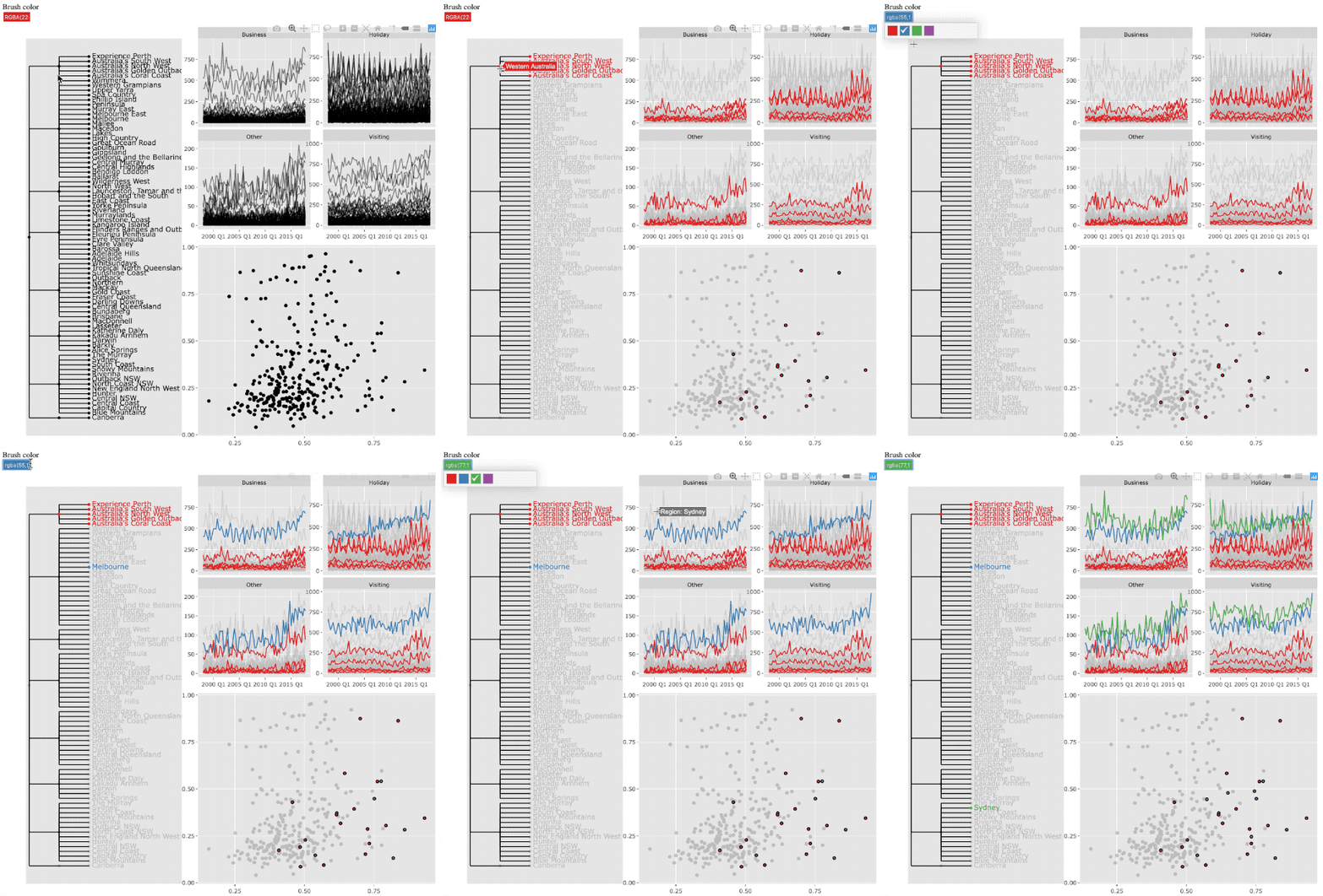
Multiple displays are constructed: (1) the overall tree plot in the
left panel, (2) the time series plot in the top right, and (3) the
scatterplot representing featured metrics for each series, produced by
the features(). All known functions here, but (yes)
generate linking views.
library(feasts)
tourism_feat <- tourism_shared %>%
  features(Trips, feat_stl)

library(ggplot2)
p1 <- tourism_shared %>%
  ggplot(aes(x = Quarter, y = Trips)) +
  geom_line(aes(group = Region), alpha = 0.5) +
  facet_wrap(~ Purpose, scales = "free_y")
p2 <- tourism_feat %>%
  ggplot(aes(x = trend_strength, y = seasonal_strength_year)) +
  geom_point(aes(group = Region))

library(plotly)
subplot(p0,
  subplot(
    ggplotly(p1, tooltip = "Region", width = 900),
    ggplotly(p2, tooltip = "Region", width = 900),
    nrows = 2),
  widths = c(.4, .6)) %>%
  highlight(dynamic = TRUE)
The key carries nested and crossed embedding, and the
index provides temporal information. Slicing and dicing
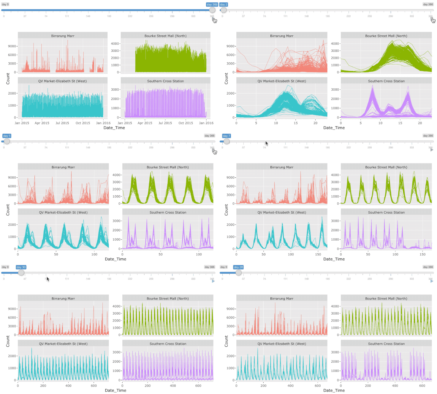
time index can help to build richer profiles for each series. A shiny
module, a pair of UI and server functions, is provided to interactively
slice and dice a tsibble. This allows to quickly locate an
interesting slice in time.
p <- fill_gaps(pedestrian) %>%
  filter_index(~ "2015") %>%
  ggplot(aes(x = Date_Time, y = Count, colour = Sensor)) +
  geom_line(size = .2) +
  facet_wrap(~ Sensor, scales = "free_y") +
  theme(legend.position = "none")

library(shiny)
ui <- fluidPage(tsibbleWrapUI("tswrap"))
server <- function(input, output, session) {
  tsibbleWrapServer("tswrap", p, period = "1 day")
}
shinyApp(ui, server)