![]()
![]()
![]()

visdat is available on CRAN
install.packages("visdat")If you would like to use the development version, install from github with:
# install.packages("devtools")
devtools::install_github("ropensci/visdat")Initially inspired by csv-fingerprint,
vis_dat helps you visualise a dataframe and “get a look at
the data” by displaying the variable classes in a dataframe as a plot
with vis_dat, and getting a brief look into missing data
patterns using vis_miss.
visdat has 6 functions:
vis_dat() visualises a dataframe showing you what
the classes of the columns are, and also displaying the missing
data.
vis_miss() visualises just the missing data, and
allows for missingness to be clustered and columns rearranged.
vis_miss() is similar to missing.pattern.plot
from the mi
package. Unfortunately missing.pattern.plot is no longer in
the mi package (as of 14/02/2016).
vis_compare() visualise differences between two
dataframes of the same dimensions
vis_expect() visualise where certain conditions hold
true in your data
vis_cor() visualise the correlation of variables in
a nice heatmap
vis_guess() visualise the individual class of each
value in your data
vis_value() visualise the value class of each cell
in your data
vis_binary() visualise the occurrence of binary
values in your data
You can read more about visdat in the vignette, [“using visdat”]https://docs.ropensci.org/visdat/articles/using_visdat.html).
Please note that the visdat project is released with a Contributor Code of Conduct. By contributing to this project, you agree to abide by its terms.
vis_dat()Let’s see what’s inside the airquality dataset from base
R, which contains information about daily air quality measurements in
New York from May to September 1973. More information about the dataset
can be found with ?airquality.
library(visdat)

vis_dat(airquality)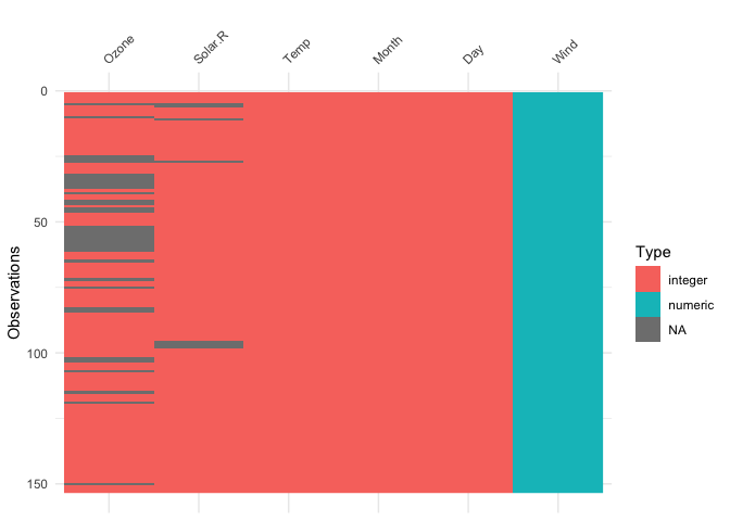
The plot above tells us that R reads this dataset as having numeric
and integer values, with some missing data in Ozone and
Solar.R. The classes are represented on the legend, and
missing data represented by grey. The column/variable names are listed
on the x axis.
The vis_dat() function also has a facet
argument, so you can create small multiples of a similar plot for a
level of a variable, e.g., Month:
vis_dat(airquality, facet = Month)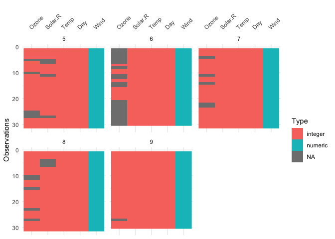
These currently also exist for vis_miss(), and the
vis_cor() functions.
vis_miss()We can explore the missing data further using
vis_miss():
vis_miss(airquality)
Percentages of missing/complete in vis_miss are accurate
to the integer (whole number). To get more accurate and thorough
exploratory summaries of missingness, I would recommend the naniar R
package
You can cluster the missingness by setting
cluster = TRUE:
vis_miss(airquality,
         cluster = TRUE)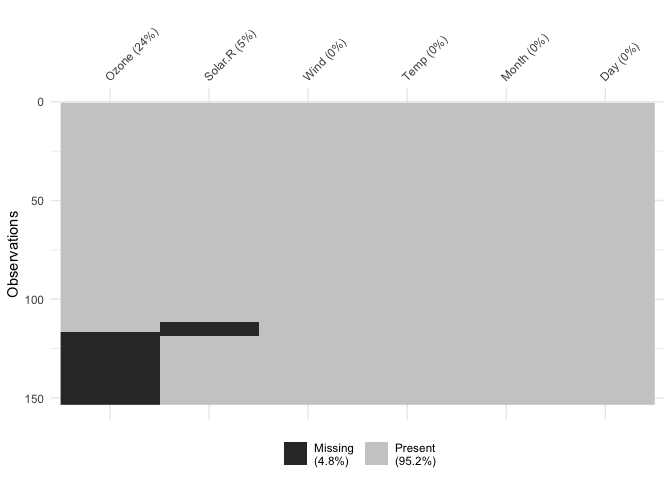
Columns can also be arranged by columns with most missingness, by
setting sort_miss = TRUE:
vis_miss(airquality,
         sort_miss = TRUE)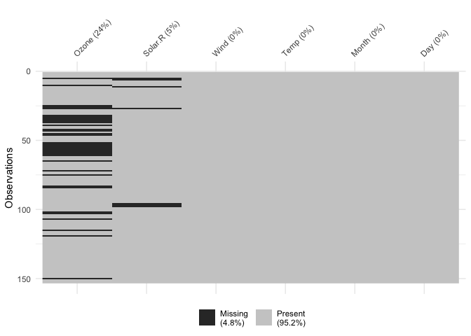
vis_miss indicates when there is a very small amount of
missing data at <0.1% missingness:
test_miss_df <- data.frame(x1 = 1:10000,
                           x2 = rep("A", 10000),
                           x3 = c(rep(1L, 9999), NA))

vis_miss(test_miss_df)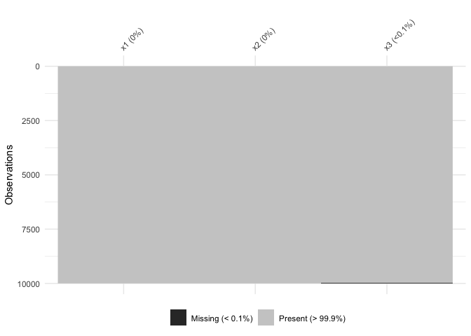
vis_miss will also indicate when there is no missing
data at all:
vis_miss(mtcars)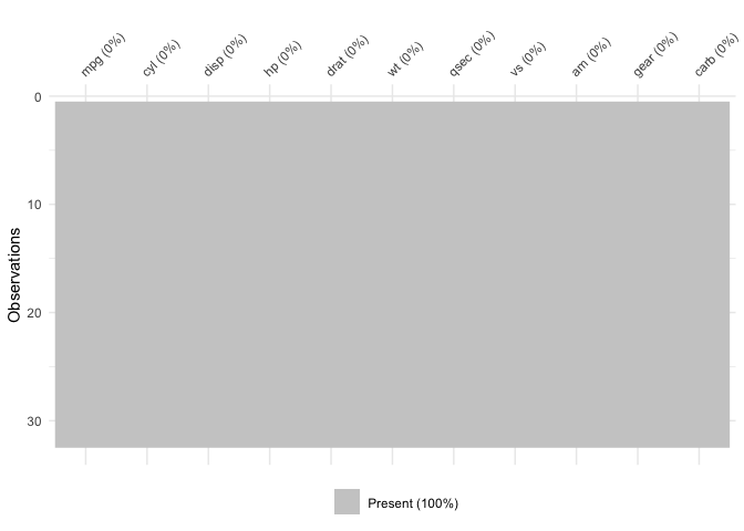
To further explore the missingness structure in a dataset, I
recommend the naniar
package, which provides more general tools for graphical and numerical
exploration of missing values.
vis_compare()Sometimes you want to see what has changed in your data.
vis_compare() displays the differences in two dataframes of
the same size. Let’s look at an example.
Let’s make some changes to the chickwts, and compare
this new dataset:
set.seed(2019-04-03-1105)
chickwts_diff <- chickwts
chickwts_diff[sample(1:nrow(chickwts), 30),sample(1:ncol(chickwts), 2)] <- NA

vis_compare(chickwts_diff, chickwts)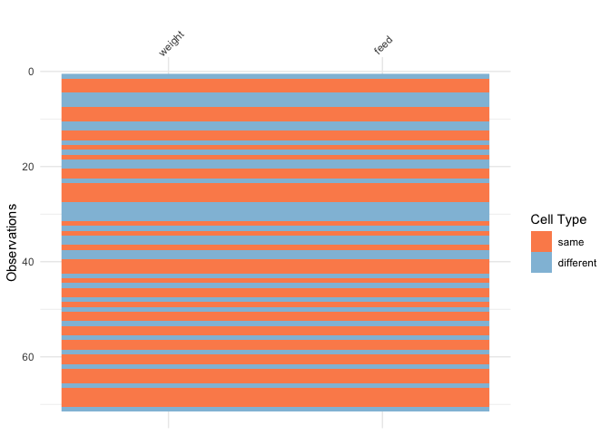
Here the differences are marked in blue.
If you try and compare differences when the dimensions are different, you get an ugly error:
chickwts_diff_2 <- chickwts
chickwts_diff_2$new_col <- chickwts_diff_2$weight*2

vis_compare(chickwts, chickwts_diff_2)
# Error in vis_compare(chickwts, chickwts_diff_2) :
# Dimensions of df1 and df2 are not the same. vis_compare requires dataframes of identical dimensions.vis_expect()vis_expect visualises certain conditions or values in
your data. For example, If you are not sure whether to expect values
greater than 25 in your data (airquality), you could write:
vis_expect(airquality, ~.x>=25), and you can see if
there are times where the values in your data are greater than or equal
to 25:
vis_expect(airquality, ~.x >= 25)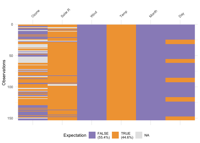
This shows the proportion of times that there are values greater than 25, as well as the missings.
vis_cor()To make it easy to plot correlations of your data, use
vis_cor:
vis_cor(airquality)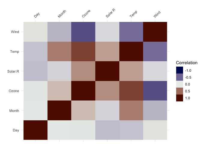
vis_valuevis_value() visualises the values of your data on a 0 to
1 scale.
vis_value(airquality)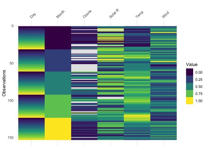
It only works on numeric data, so you might get strange results if you are using factors:
library(ggplot2)
vis_value(iris)
data input can only contain numeric values, please subset the data to the numeric values you would like. dplyr::select_if(data, is.numeric) can be helpful here!So you might need to subset the data beforehand like so:
library(dplyr)
#>
#> Attaching package: 'dplyr'
#> The following objects are masked from 'package:stats':
#>
#>     filter, lag
#> The following objects are masked from 'package:base':
#>
#>     intersect, setdiff, setequal, union

iris %>%
  select_if(is.numeric) %>%
  vis_value()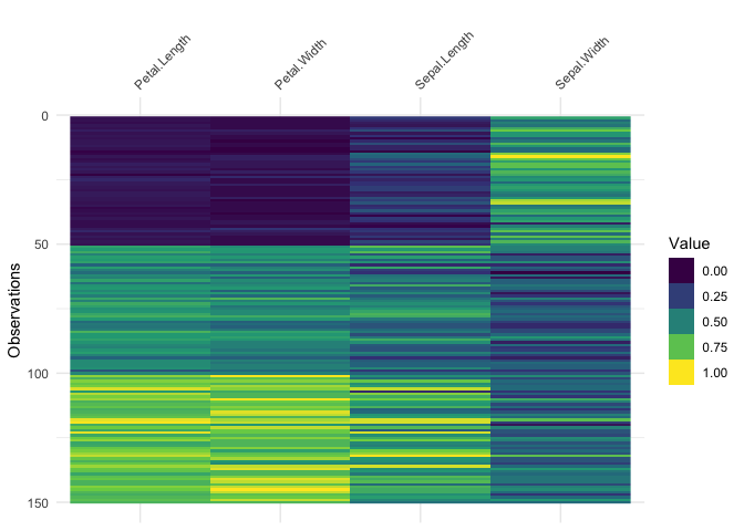
vis_binary()vis_binary() visualises binary values. See below for use
with example data, dat_bin
vis_binary(dat_bin)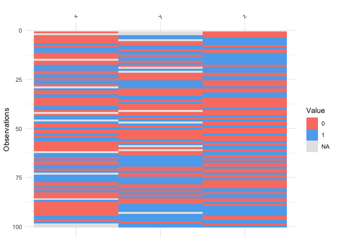
If you don’t have only binary values a warning will be shown.
vis_binary(airquality)Error in test_if_all_binary(data) :
data input can only contain binary values - this means either 0 or 1, or NA. Please subset the data to be binary values, or see ?vis_value.vis_guess()vis_guess() takes a guess at what each cell is. It’s
best illustrated using some messy data, which we’ll make here:
messy_vector <- c(TRUE,
                  T,
                  "TRUE",
                  "T",
                  "01/01/01",
                  "01/01/2001",
                  NA,
                  NaN,
                  "NA",
                  "Na",
                  "na",
                  "10",
                  10,
                  "10.1",
                  10.1,
                  "abc",
                  "$%TG")

set.seed(2019-04-03-1106)
messy_df <- data.frame(var1 = messy_vector,
                       var2 = sample(messy_vector),
                       var3 = sample(messy_vector))
vis_guess(messy_df)
vis_dat(messy_df)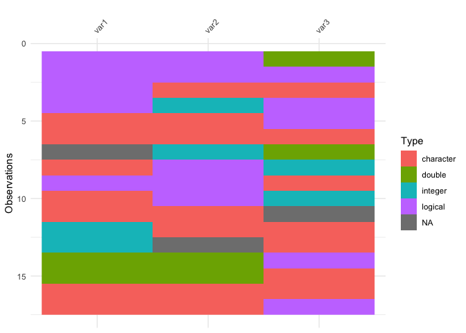
So here we see that there are many different kinds of data in your dataframe. As an analyst this might be a depressing finding. We can see this comparison above.
Thank you to Ivan Hanigan who first
commented this suggestion after I made a blog post about an initial
prototype ggplot_missing, and Jenny Bryan, whose tweet
got me thinking about vis_dat, and for her code
contributions that removed a lot of errors.
Thank you to Hadley Wickham for suggesting the use of the internals
of readr to make vis_guess work. Thank you to
Miles McBain for his suggestions on how to improve
vis_guess. This resulted in making it at least 2-3 times
faster. Thanks to Carson Sievert for writing the code that combined
plotly with visdat, and for Noam Ross for
suggesting this in the first place. Thank you also to Earo Wang and
Stuart Lee for their help in getting capturing expressions in
vis_expect.
Finally thank you to rOpenSci and it’s amazing onboarding process, this process has made visdat a much better package, thanks to the editor Noam Ross (@noamross), and the reviewers Sean Hughes (@seaaan) and Mara Averick (@batpigandme).